Note
Click here to download the full example code
09. Triangular grids with mpl.tripcolor
This script demonstrates how to visualize data on an unstructured
triangular grid using matplotlib.tripcolor. This is useful
for plotting data that is not arranged in a regular grid.
The example covers two main scenarios:
Automatically creating a Delaunay triangulation from a set of 2D points.
Plotting data on a pre-defined, user-specified mesh of triangles.
It also compares flat and gouraud shading methods.
Out:
C:\Users\kelda\Desktop\repositories\github\python-spare-code\main\examples\matplotlib\plot_main09_tripcolor.py:112: UserWarning:

FigureCanvasAgg is non-interactive, and thus cannot be shown
18 import matplotlib.pyplot as plt
19 import matplotlib.tri as tri
20 import numpy as np
21
22 # First create the x and y coordinates of the points.
23 n_angles = 36
24 n_radii = 8
25 min_radius = 0.25
26 radii = np.linspace(min_radius, 0.95, n_radii)
27
28 angles = np.linspace(0, 2 * np.pi, n_angles, endpoint=False)
29 angles = np.repeat(angles[..., np.newaxis], n_radii, axis=1)
30 angles[:, 1::2] += np.pi / n_angles
31
32 x = (radii * np.cos(angles)).flatten()
33 y = (radii * np.sin(angles)).flatten()
34 z = (np.cos(radii) * np.cos(3 * angles)).flatten()
35
36 # Create the Triangulation; no triangles so Delaunay triangulation created.
37 triang = tri.Triangulation(x, y)
38
39 # Mask off unwanted triangles.
40 triang.set_mask(np.hypot(x[triang.triangles].mean(axis=1),
41 y[triang.triangles].mean(axis=1))
42 < min_radius)
43
44 fig1, ax1 = plt.subplots()
45 ax1.set_aspect('equal')
46 tpc = ax1.tripcolor(triang, z, shading='flat')
47 fig1.colorbar(tpc)
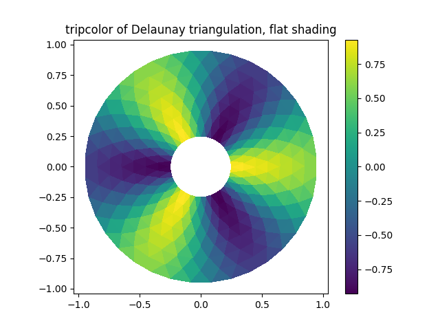
48 ax1.set_title('tripcolor of Delaunay triangulation, flat shading')
49
50 fig2, ax2 = plt.subplots()
51 ax2.set_aspect('equal')
52 tpc = ax2.tripcolor(triang, z, shading='gouraud')
53 fig2.colorbar(tpc)
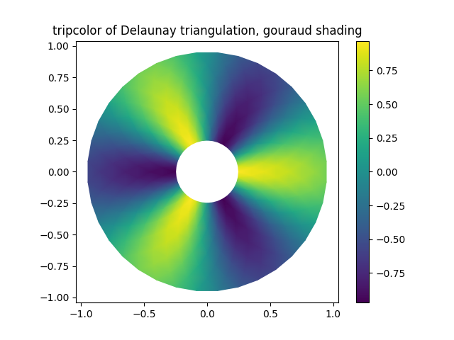
54 ax2.set_title('tripcolor of Delaunay triangulation, gouraud shading')
55
56
57 xy = np.asarray([
58 [-0.101, 0.872], [-0.080, 0.883], [-0.069, 0.888], [-0.054, 0.890],
59 [-0.045, 0.897], [-0.057, 0.895], [-0.073, 0.900], [-0.087, 0.898],
60 [-0.090, 0.904], [-0.069, 0.907], [-0.069, 0.921], [-0.080, 0.919],
61 [-0.073, 0.928], [-0.052, 0.930], [-0.048, 0.942], [-0.062, 0.949],
62 [-0.054, 0.958], [-0.069, 0.954], [-0.087, 0.952], [-0.087, 0.959],
63 [-0.080, 0.966], [-0.085, 0.973], [-0.087, 0.965], [-0.097, 0.965],
64 [-0.097, 0.975], [-0.092, 0.984], [-0.101, 0.980], [-0.108, 0.980],
65 [-0.104, 0.987], [-0.102, 0.993], [-0.115, 1.001], [-0.099, 0.996],
66 [-0.101, 1.007], [-0.090, 1.010], [-0.087, 1.021], [-0.069, 1.021],
67 [-0.052, 1.022], [-0.052, 1.017], [-0.069, 1.010], [-0.064, 1.005],
68 [-0.048, 1.005], [-0.031, 1.005], [-0.031, 0.996], [-0.040, 0.987],
69 [-0.045, 0.980], [-0.052, 0.975], [-0.040, 0.973], [-0.026, 0.968],
70 [-0.020, 0.954], [-0.006, 0.947], [ 0.003, 0.935], [ 0.006, 0.926],
71 [ 0.005, 0.921], [ 0.022, 0.923], [ 0.033, 0.912], [ 0.029, 0.905],
72 [ 0.017, 0.900], [ 0.012, 0.895], [ 0.027, 0.893], [ 0.019, 0.886],
73 [ 0.001, 0.883], [-0.012, 0.884], [-0.029, 0.883], [-0.038, 0.879],
74 [-0.057, 0.881], [-0.062, 0.876], [-0.078, 0.876], [-0.087, 0.872],
75 [-0.030, 0.907], [-0.007, 0.905], [-0.057, 0.916], [-0.025, 0.933],
76 [-0.077, 0.990], [-0.059, 0.993]])
77 x, y = np.rad2deg(xy).T
78
79 triangles = np.asarray([
80 [67, 66, 1], [65, 2, 66], [ 1, 66, 2], [64, 2, 65], [63, 3, 64],
81 [60, 59, 57], [ 2, 64, 3], [ 3, 63, 4], [ 0, 67, 1], [62, 4, 63],
82 [57, 59, 56], [59, 58, 56], [61, 60, 69], [57, 69, 60], [ 4, 62, 68],
83 [ 6, 5, 9], [61, 68, 62], [69, 68, 61], [ 9, 5, 70], [ 6, 8, 7],
84 [ 4, 70, 5], [ 8, 6, 9], [56, 69, 57], [69, 56, 52], [70, 10, 9],
85 [54, 53, 55], [56, 55, 53], [68, 70, 4], [52, 56, 53], [11, 10, 12],
86 [69, 71, 68], [68, 13, 70], [10, 70, 13], [51, 50, 52], [13, 68, 71],
87 [52, 71, 69], [12, 10, 13], [71, 52, 50], [71, 14, 13], [50, 49, 71],
88 [49, 48, 71], [14, 16, 15], [14, 71, 48], [17, 19, 18], [17, 20, 19],
89 [48, 16, 14], [48, 47, 16], [47, 46, 16], [16, 46, 45], [23, 22, 24],
90 [21, 24, 22], [17, 16, 45], [20, 17, 45], [21, 25, 24], [27, 26, 28],
91 [20, 72, 21], [25, 21, 72], [45, 72, 20], [25, 28, 26], [44, 73, 45],
92 [72, 45, 73], [28, 25, 29], [29, 25, 31], [43, 73, 44], [73, 43, 40],
93 [72, 73, 39], [72, 31, 25], [42, 40, 43], [31, 30, 29], [39, 73, 40],
94 [42, 41, 40], [72, 33, 31], [32, 31, 33], [39, 38, 72], [33, 72, 38],
95 [33, 38, 34], [37, 35, 38], [34, 38, 35], [35, 37, 36]])
96
97 xmid = x[triangles].mean(axis=1)
98 ymid = y[triangles].mean(axis=1)
99 x0 = -5
100 y0 = 52
101 zfaces = np.exp(-0.01 * ((xmid - x0) * (xmid - x0) +
102 (ymid - y0) * (ymid - y0)))
103
104 fig3, ax3 = plt.subplots()
105 ax3.set_aspect('equal')
106 tpc = ax3.tripcolor(x, y, triangles, facecolors=zfaces, edgecolors='k')
107 fig3.colorbar(tpc)
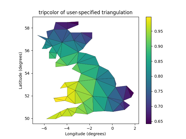
108 ax3.set_title('tripcolor of user-specified triangulation')
109 ax3.set_xlabel('Longitude (degrees)')
110 ax3.set_ylabel('Latitude (degrees)')
111
112 plt.show()
Total running time of the script: ( 0 minutes 0.284 seconds)