07.d stats.2dbin with shap.csv

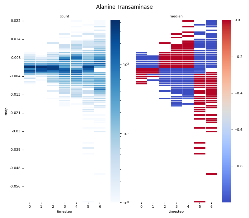
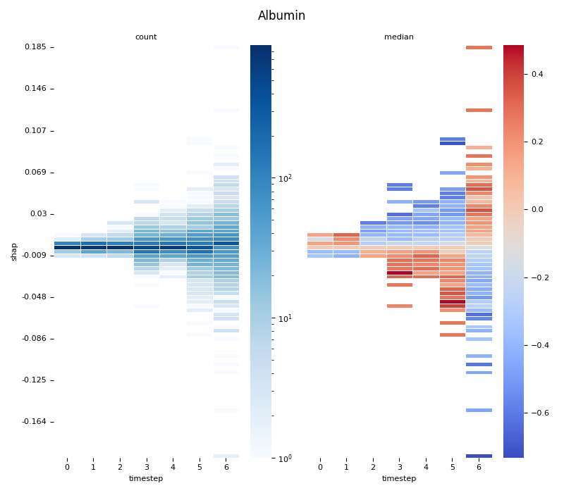
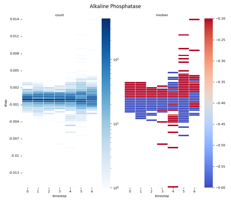
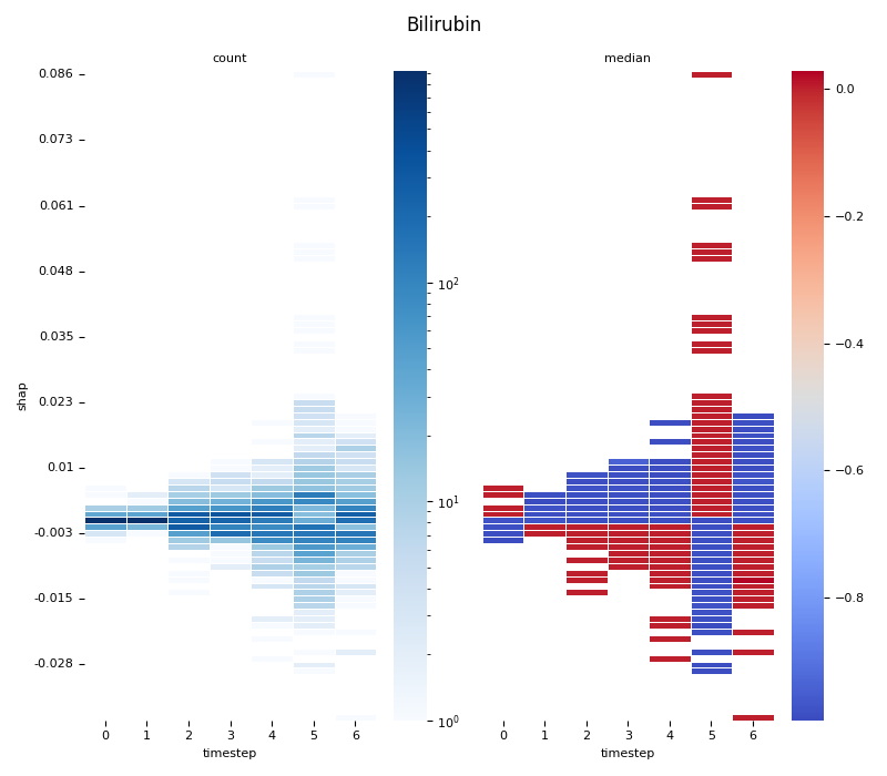
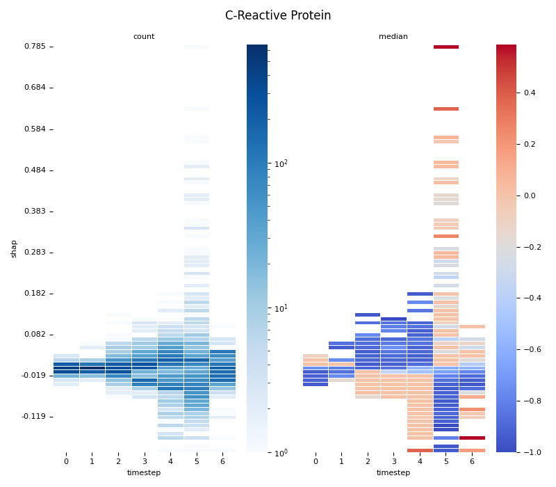
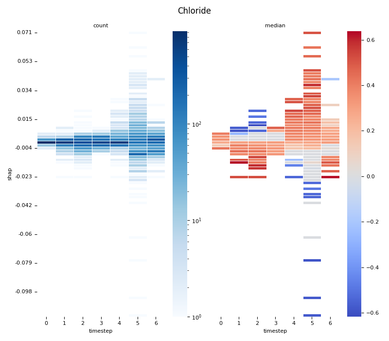
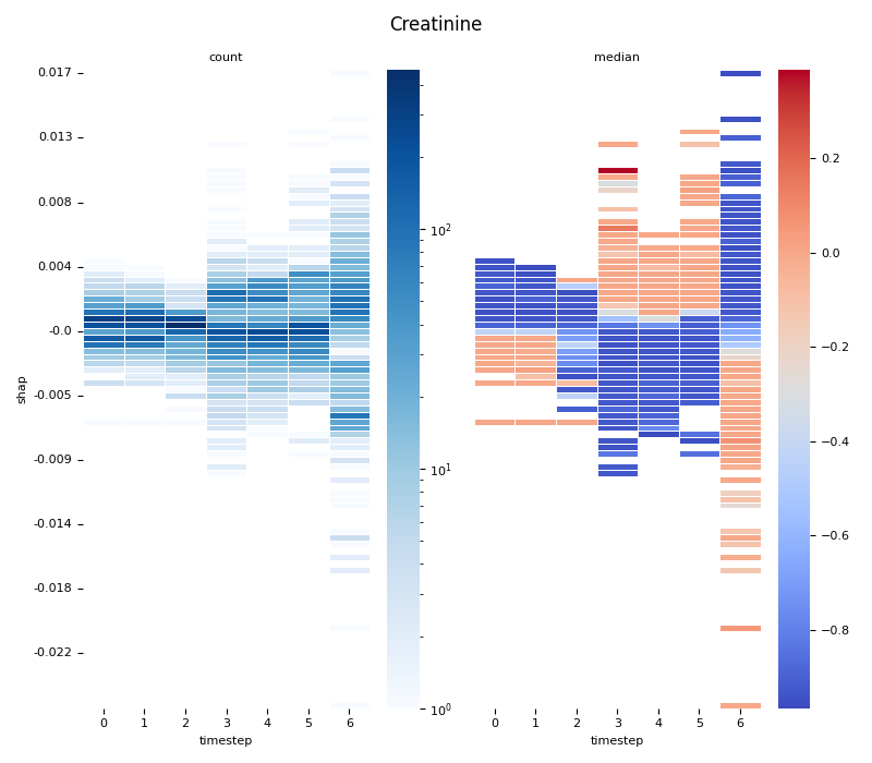
This script provides an advanced, per-feature analysis of time-series SHAP data, creating a dual-heatmap visualization to reveal complex interactions between feature values, their SHAP importance, and time. 📊

The workflow includes:

• Per-Feature Processing: It iterates through individual features from a pre-computed SHAP dataset.

• Statistical Binning: For each feature, it uses scipy.stats.binned_statistic_2d to compute both the count of data points and the median of the original feature values for each cell in a 2D grid.

• Dual Heatmap Visualization: It plots two heatmaps side-by-side: one showing data density (with a log scale) and the other showing the median feature value (with a diverging colormap), allowing for direct comparison.

• 
• 
• 
• 
• 
• 
• 

Out:

    Unnamed: 0  sample  timestep              features  feature_values  shap_values
12          12       0         0            Creatinine             0.0    -0.001081
17          17       0         0              Chloride             0.0    -0.000858
21          21       0         0    C-Reactive Protein             0.0     0.010186
22          22       0         0               Albumin             0.0     0.000411
23          23       0         0  Alkaline Phosphatase             0.0     0.000486
27          27       0         0  Alanine Transaminase             0.0    -0.001809
28          28       0         0             Bilirubin             0.0     0.000500
48          48       0         1            Creatinine             0.0    -0.001033
53          53       0         1              Chloride             0.0     0.001109
57          57       0         1    C-Reactive Protein             0.0     0.005363
 0. Computing... Alanine Transaminase
 1. Computing... Albumin
 2. Computing... Alkaline Phosphatase
 3. Computing... Bilirubin
 4. Computing... C-Reactive Protein
 5. Computing... Chloride
 6. Computing... Creatinine
C:\Users\kelda\Desktop\repositories\github\python-spare-code\main\examples\matplotlib\plot_main07_d_2dbin_shap.py:173: UserWarning:

FigureCanvasAgg is non-interactive, and thus cannot be shown

# Libraries
import seaborn as sns
import pandas as pd
import numpy as np
import matplotlib as mpl
import matplotlib.pyplot as plt

from scipy import stats
from pathlib import Path
from matplotlib.colors import LogNorm

#plt.style.use('ggplot') # R ggplot style

# See https://matplotlib.org/devdocs/users/explain/customizing.html
mpl.rcParams['axes.titlesize'] = 8
mpl.rcParams['axes.labelsize'] = 8
mpl.rcParams['xtick.labelsize'] = 8
mpl.rcParams['ytick.labelsize'] = 8

# Constant
SNS_HEATMAP_CBAR_ARGS = {
    'C-Reactive Protein': { 'vmin':-0.4, 'vmax':-0.2, 'center':-0.35 },
    'Bilirubin': { 'vmin':-0.4, 'vmax':-0.2, 'center':-0.35 },
    'Alanine Transaminase': {},
    'Albumin': {},
    'Alkaline Phosphatase': { 'vmin':-0.6, 'vmax':-0.2 },
    'Bilirubin': {},
    'C-Reactive Protein': {},
    'Chloride': {},
}

# Load data
path = Path('../../datasets/shap/')
data = pd.read_csv(path / 'shap.csv')

# Filter
data = data[data.features.isin([
    'Alanine Transaminase',
    'Albumin',
    'Alkaline Phosphatase',
    'Bilirubin',
    'C-Reactive Protein',
    'Chloride',
    'Creatinine'
])]

# Show
print(data.head(10))

# figsize = (8,7) for 100 bins
# figsize = (8,3) for 50 bins
#
# .. note: The y-axis does not represent a continuous space,
#          it is a discrete space where each tick is describing
#          a bin.

# Loop
for i, (name, df) in enumerate(data.groupby('features')):

    # Info
    print("%2d. Computing... %s" % (i, name))

    # Get variables
    x = df.timestep
    y = df.shap_values
    z = df.feature_values
    n = x.max()
    vmin = z.min()
    vmax = z.max()
    nbins = 100
    figsize = (8, 7)

    # Create bins
    binx = np.arange(x.min(), x.max()+2, 1) - 0.5
    biny = np.linspace(y.min(), y.max(), nbins)

    # Compute binned statistic (count)
    r1 = stats.binned_statistic_2d(x=y, y=x, values=z,
        statistic='count', bins=[biny, binx],
        expand_binnumbers=False)

    # Compute binned statistic (median)
    r2 = stats.binned_statistic_2d(x=y, y=x, values=z,
        statistic='median', bins=[biny, binx],
        expand_binnumbers=False)

    # Compute centres
    x_center = (r1.x_edge[:-1] + r1.x_edge[1:]) / 2
    y_center = (r1.y_edge[:-1] + r1.y_edge[1:]) / 2

    # Flip
    flip1 = np.flip(r1.statistic, 0)
    flip2 = np.flip(r2.statistic, 0)

    # Display
    fig, axs = plt.subplots(nrows=1, ncols=2,
        sharey=True, sharex=False, figsize=figsize)

    sns.heatmap(flip1, annot=False, linewidth=0.5,
                xticklabels=y_center.astype(int),
                yticklabels=x_center.round(3)[::-1],  # Because of flip
                cmap='Blues', ax=axs[0], norm=LogNorm(),
                cbar_kws={
                    #'label': 'value [unit]',
                    'use_gridspec': True,
                    'location': 'right'
                }
    )

    sns.heatmap(flip2, annot=False, linewidth=0.5,
                xticklabels=y_center.astype(int),
                yticklabels=x_center.round(3)[::-1],  # Because of flip
                cmap='coolwarm', ax=axs[1], zorder=1,
                **SNS_HEATMAP_CBAR_ARGS.get(name, {}),
                #vmin=vmin, vmax=vmax, center=center, robust=False,
                cbar_kws={
                    #'label': 'value [unit]',
                    'use_gridspec': True,
                    'location': 'right'
                }
    )

    # Configure ax0
    axs[0].set_title('count')
    axs[0].set_xlabel('timestep')
    axs[0].set_ylabel('shap')
    axs[0].locator_params(axis='y', nbins=10)

    # Configure ax1
    axs[1].set_title('median')
    axs[1].set_xlabel('timestep')
    #axs[1].set_ylabel('shap')
    axs[1].locator_params(axis='y', nbins=10)
    axs[1].tick_params(axis=u'y', which=u'both', length=0)
    # axs[1].invert_yaxis()

    # Identify zero crossing
    #zero_crossing = np.where(np.diff(np.sign(biny)))[0]
    # Display line on that index (not exactly 0 though)
    #plt.axhline(y=len(biny) - zero_crossing, color='lightgray', linestyle='--')

    # Generic
    plt.suptitle(name)
    plt.tight_layout()

    # Show only first N
    if int(i) > 5:
     break

# Show
plt.show()