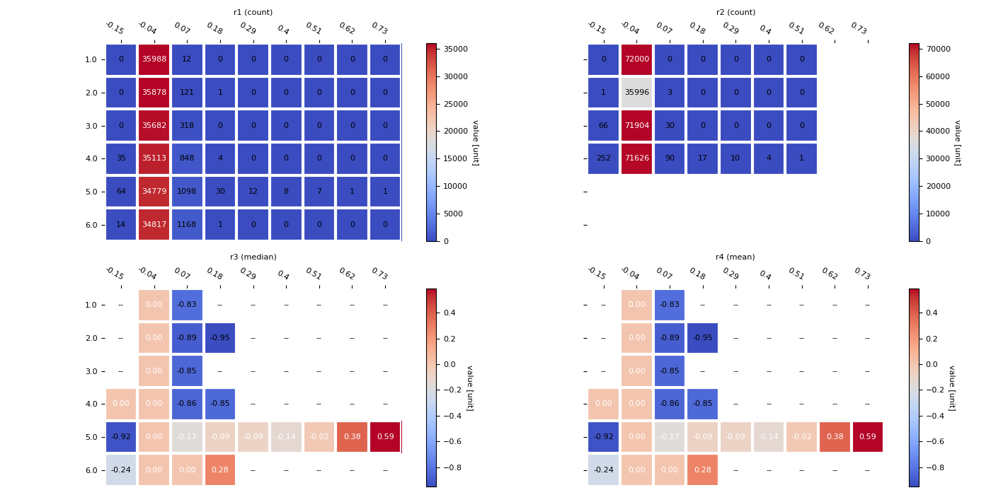
07.a stats.2dbin and mpl.heatmap

This script demonstrates how to aggregate 2D data using scipy.stats.binned_statistic_2d and then visualize the result as a detailed, annotated heatmap.

It provides a comprehensive workflow that includes:

• Binning Data: It groups scattered 2D points into a grid and computes statistics like count, median, and mean for the values within each bin.

• Custom Heatmap Function: It uses custom helper functions to build a polished heatmap from scratch using matplotlib, complete with annotations for each cell.

Out:

        Unnamed: 0  sample  timestep                       features  feature_values  shap_values
0                0       0         0                   Ward Lactate        0.000000     0.000652
1                1       0         0                   Ward Glucose        0.000000    -0.000596
2                2       0         0                       Ward sO2        0.000000     0.000231
3                3       0         0  White blood cell count, blood        0.000000     0.000582
4                4       0         0                      Platelets        0.000000    -0.001705
...            ...     ...       ...                            ...             ...          ...
251995      251995     999         6                  Procalcitonin        0.000000     0.000027
251996      251996     999         6                       Ferritin        0.000000    -0.001375
251997      251997     999         6                        D-Dimer        0.000000     0.000045
251998      251998     999         6                            sex       -1.000000    -0.002359
251999      251999     999         6                            age        0.169952     0.000237

[252000 rows x 6 columns]
C:\Users\kelda\Desktop\repositories\virtualenvs\venv-py311-psc\Lib\site-packages\matplotlib\colors.py:2242: UserWarning:

Warning: converting a masked element to nan.

C:\Users\kelda\Desktop\repositories\virtualenvs\venv-py311-psc\Lib\site-packages\matplotlib\colors.py:2249: UserWarning:

Warning: converting a masked element to nan.

C:\Users\kelda\AppData\Local\Programs\Python\Python311\Lib\string.py:264: FutureWarning:

Format strings passed to MaskedConstant are ignored, but in future may error or produce different behavior

C:\Users\kelda\Desktop\repositories\virtualenvs\venv-py311-psc\Lib\site-packages\matplotlib\colors.py:2242: UserWarning:

Warning: converting a masked element to nan.

C:\Users\kelda\Desktop\repositories\virtualenvs\venv-py311-psc\Lib\site-packages\matplotlib\colors.py:2249: UserWarning:

Warning: converting a masked element to nan.

C:\Users\kelda\AppData\Local\Programs\Python\Python311\Lib\string.py:264: FutureWarning:

Format strings passed to MaskedConstant are ignored, but in future may error or produce different behavior

C:\Users\kelda\Desktop\repositories\github\python-spare-code\main\examples\matplotlib\plot_main07_a_2dbin_stat.py:256: UserWarning:

FigureCanvasAgg is non-interactive, and thus cannot be shown

import matplotlib
import numpy as np
import pandas as pd
import matplotlib as mpl
import matplotlib.pyplot as plt

from scipy import stats

# See https://matplotlib.org/devdocs/users/explain/customizing.html
mpl.rcParams['font.size'] = 8
mpl.rcParams['axes.titlesize'] = 8
mpl.rcParams['axes.labelsize'] = 8
mpl.rcParams['xtick.labelsize'] = 8
mpl.rcParams['ytick.labelsize'] = 8

def heatmap(data, row_labels, col_labels, ax=None,
            cbar_kw=None, cbarlabel="", **kwargs):
    """
    Create a heatmap from a numpy array and two lists of labels.

    Parameters
    ----------
    data
        A 2D numpy array of shape (M, N).
    row_labels
        A list or array of length M with the labels for the rows.
    col_labels
        A list or array of length N with the labels for the columns.
    ax
        A `matplotlib.axes.Axes` instance to which the heatmap is plotted.  If
        not provided, use current axes or create a new one.  Optional.
    cbar_kw
        A dictionary with arguments to `matplotlib.Figure.colorbar`.  Optional.
    cbarlabel
        The label for the colorbar.  Optional.
    **kwargs
        All other arguments are forwarded to `imshow`.
    """

    if ax is None:
        ax = plt.gca()

    if cbar_kw is None:
        cbar_kw = {}

    # Plot the heatmap
    im = ax.imshow(data, **kwargs)

    # Create colorbar
    cbar = ax.figure.colorbar(im, ax=ax, **cbar_kw)
    cbar.ax.set_ylabel(cbarlabel, rotation=-90, va="bottom")

    # Show all ticks and label them with the respective list entries.
    ax.set_xticks(np.arange(data.shape[1]), labels=col_labels)
    ax.set_yticks(np.arange(data.shape[0]), labels=row_labels)

    # Let the horizontal axes labeling appear on top.
    ax.tick_params(top=True, bottom=False,
                   labeltop=True, labelbottom=False)

    # Rotate the tick labels and set their alignment.
    plt.setp(ax.get_xticklabels(), rotation=-30, ha="right",
             rotation_mode="anchor")

    # Turn spines off and create white grid.
    ax.spines[:].set_visible(False)

    ax.set_xticks(np.arange(data.shape[1]+1)-.5, minor=True)
    ax.set_yticks(np.arange(data.shape[0]+1)-.5, minor=True)
    ax.grid(which="minor", color="w", linestyle='-', linewidth=3)
    ax.tick_params(which="minor", bottom=False, left=False)

    return im, cbar


def annotate_heatmap(im, data=None, valfmt="{x:.2f}",
                     textcolors=("black", "white"),
                     threshold=None, **textkw):
    """
    A function to annotate a heatmap.

    Parameters
    ----------
    im
        The AxesImage to be labeled.
    data
        Data used to annotate.  If None, the image's data is used.  Optional.
    valfmt
        The format of the annotations inside the heatmap.  This should either
        use the string format method, e.g. "$ {x:.2f}", or be a
        `matplotlib.ticker.Formatter`.  Optional.
    textcolors
        A pair of colors.  The first is used for values below a threshold,
        the second for those above.  Optional.
    threshold
        Value in data units according to which the colors from textcolors are
        applied.  If None (the default) uses the middle of the colormap as
        separation.  Optional.
    **kwargs
        All other arguments are forwarded to each call to `text` used to create
        the text labels.
    """

    if not isinstance(data, (list, np.ndarray)):
        data = im.get_array()

    # Normalize the threshold to the images color range.
    if threshold is not None:
        threshold = im.norm(threshold)
    else:
        threshold = im.norm(data.max())/2.

    # Set default alignment to center, but allow it to be
    # overwritten by textkw.
    kw = dict(horizontalalignment="center",
              verticalalignment="center")
    kw.update(textkw)

    # Get the formatter in case a string is supplied
    if isinstance(valfmt, str):
        valfmt = matplotlib.ticker.StrMethodFormatter(valfmt)

    # Loop over the data and create a `Text` for each "pixel".
    # Change the text's color depending on the data.
    texts = []
    for i in range(data.shape[0]):
        for j in range(data.shape[1]):
            kw.update(color=textcolors[int(im.norm(data[i, j]) > threshold)])
            text = im.axes.text(j, i, valfmt(data[i, j], None), **kw)
            texts.append(text)

    return texts


def plot_binned_statistic(r, ax, title=None, astype=None, **kwargs):
    """Plots the binned statistic

    Parameters
    ----------
    r: the binned statistic
    ax: the axes to plot

    Returns
    -------
    """
    # Variables
    rows, cols = r.statistic.shape

    # Compute centers
    x_center = (r.x_edge[:-1] + r.x_edge[1:]) / 2
    y_center = (r.y_edge[:-1] + r.y_edge[1:]) / 2

    # Plot heatmap (matplotlib sample, use seaborn instead)
    im, cbar = heatmap(r.statistic,
        np.around(x_center, 2), np.around(y_center, 2), ax=ax,
        cmap="coolwarm", cbarlabel="value [unit]")
    texts = annotate_heatmap(im, **kwargs)

    # Configure
    ax.set_aspect('equal', 'box')
    if title is not None:
        ax.set_title(title)

    """
    # Show
    print("\n\n")
    print(matrix)
    print(r.x_edge)
    print(r.y_edge)
    print(r.binnumber)
    print(np.flip(r.statistic, axis=1))
    """

def data_manual():
    """"""
    # Create random values
    x = np.array([1, 1, 1, 1, 2, 2, 2, 3, 4])
    y = np.array([1, 1, 2, 2, 3, 4, 5, 6, 7])
    z = np.array([1, 9, 9, 1, 2, 2, 2, 3, 4])
    return x, y, z

def data_shap():
    """"""
    data = pd.read_csv('../../datasets/shap/shap.csv')
    print(data)
    return data.timestep, data.shap_values, data.feature_values




# Load data
#x, y, z = data_manual()
x, y, z = data_shap()

# Using np.arange
binx = np.arange(0, x.max()+1) + 0.5 # [0.5, 1.5, 2.5, ...., N + 0.5]
biny = np.arange(0, y.max()+1) + 0.5 # [0.5, 1.5, 2.5, ...., N + 0.5]

# Using np.linspace
biny = np.linspace(y.min(), y.max(), 10)

# Manual
#binx = np.arange(5) + 0.5
#biny = np.arange(8) + 0.5

# Compute binned statistic (count)
r1 = stats.binned_statistic_2d(x=x, y=y, values=None,
    statistic='count', bins=[binx, biny],
    expand_binnumbers=True)

# Compute binned statistic (median)
r2 = stats.binned_statistic_2d(x=x, y=y, values=z,
    statistic='count', bins=[4, 7],
    expand_binnumbers=False)

# Compute binned statistic (median)
r3 = stats.binned_statistic_2d(x=x, y=y, values=z,
    statistic='median', bins=[binx, biny],
    expand_binnumbers=False)

# Compute binned statistic (median)
r4 = stats.binned_statistic_2d(x=x, y=y, values=z,
    statistic='mean', bins=[binx, biny],
    expand_binnumbers=False)


# Plot
fig, axs = plt.subplots(nrows=2, ncols=2,
    sharey=True, sharex=True, figsize=(14, 7))
plot_binned_statistic(r1, axs[0,0], title='r1 (count)', valfmt="{x:g}")
plot_binned_statistic(r2, axs[0,1], title='r2 (count)', valfmt="{x:g}")
plot_binned_statistic(r3, axs[1,0], title='r3 (median)')
plot_binned_statistic(r3, axs[1,1], title='r4 (mean)')

# Display
plt.tight_layout()
plt.show()