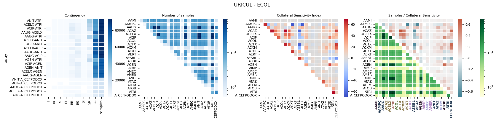
06.c Collateral Sensitivity Index (CRI)

This script creates a sophisticated, multi-panel visualization for pre-computed Collateral Sensitivity Index (CRI) data, designed for in-depth analysis of drug interactions.

The workflow includes:

• Data Loading: It ingests pre-processed CRI and sample frequency data from CSV files.

• Multi-Heatmap Layout: It generates several seaborn heatmaps: one for the CRI (using a diverging colormap), another for sample counts (with a log scale), and a composite heatmap combining both metrics in its upper and lower triangles.

• Categorical Annotation: It enhances the final plot by adding color-coded labels to the axes based on antibiotic categories, creating a dense, information-rich figure.

Note

Since the computation of the Collateral Sensitivity Index is quite computationally expensive, the results are saved into a .csv file so that can be easily loaded and displayed. This script shows a very basic graph of such information.

# Libraries
import numpy as np
import pandas as pd
import seaborn as sns
import matplotlib as mpl
import matplotlib.pyplot as plt

#
from pathlib import Path
from itertools import combinations
from matplotlib.colors import LogNorm, Normalize

# See https://matplotlib.org/devdocs/users/explain/customizing.html
mpl.rcParams['axes.titlesize'] = 8
mpl.rcParams['axes.labelsize'] = 8
mpl.rcParams['xtick.labelsize'] = 8
mpl.rcParams['ytick.labelsize'] = 8

try:
    __file__
    TERMINAL = True
except:
    TERMINAL = False


# --------------------------------
# Methods
# --------------------------------
def _check_ax_ay_equal(ax, ay):
    return ax==ay

def _check_ax_ay_greater(ax, ay):
    return  ax>ay

# --------------------------------
# Constants
# --------------------------------
# Possible cmaps
# https://r02b.github.io/seaborn_palettes/
# Diverging: coolwarm, RdBu_r, vlag
# Others: bone, gray, pink, twilight
cmap0 = 'coolwarm'
cmap1 = sns.light_palette("seagreen", as_cmap=True)
cmap2 = sns.color_palette("light:b", as_cmap=True)
cmap3 = sns.color_palette("vlag", as_cmap=True)
cmap4 = sns.diverging_palette(220, 20, as_cmap=True)
cmap5 = sns.color_palette("ch:s=.25,rot=-.25", as_cmap=True) # no
cmap6 = sns.color_palette("light:#5A9", as_cmap=True)
cmap7 = sns.light_palette("#9dedcc", as_cmap=True)
cmap8 = sns.color_palette("YlGn", as_cmap=True)

# Figure size
figsize = (17, 4)

Let’s load the data

# Load data
path = Path('../../datasets/collateral-sensitivity/20230525-135511')
data = pd.read_csv(path / 'contingency.csv')
abxs = pd.read_csv(path / 'categories.csv')

# Format data
data = data.set_index(['specimen', 'o', 'ax', 'ay'])
data.RR = data.RR.fillna(0).astype(int)
data.RS = data.RS.fillna(0).astype(int)
data.SR = data.SR.fillna(0).astype(int)
data.SS = data.SS.fillna(0).astype(int)
data['samples'] = data.RR + data.RS + data.SR + data.SS

#data['samples'] = data.iloc[:, :4].sum(axis=1)

def filter_top_pairs(df, n=5):
    """Filter top n (Specimen, Organism) pairs."""
    # Find top
    top = df.groupby(level=[0, 1]) \
        .samples.sum() \
        .sort_values(ascending=False) \
        .head(n)

    # Filter
    idx = pd.IndexSlice
    a = top.index.get_level_values(0).unique()
    b = top.index.get_level_values(1).unique()

    # Return
    return df.loc[idx[a, b, :, :]]

# Filter
data = filter_top_pairs(data, n=2)
data = data[data.samples > 500]

Lets see the data

if TERMINAL:
    print("\n")
    print("Number of samples: %s" % data.samples.sum())
    print("Number of pairs: %s" % data.shape[0])
    print("Data:")
    print(data)
data.iloc[:7,:].dropna(axis=1, how='all')

				RR	RS	SI	SR	SS	MIS	samples
specimen	o	ax	ay
WOUCUL	SAUR	ACHL	ACLI	2	10	3.0	165	585	-0.003227	762
			AERY	2	10	4.0	213	536	-0.007012	761
			AFUS	2	10	NaN	86	667	0.003373	765
			ALIN	0	10	NaN	0	523	0.000000	533
			AMET	3	9	NaN	71	679	0.010702	762
			AMUP	0	10	6.0	3	690	-0.000183	703
			ANEO	1	9	NaN	27	622	0.003881	659

Lets load the antimicrobial data and create color mapping variables

# Create dictionary to map category to color
labels = abxs.category
palette = sns.color_palette('Spectral', labels.nunique())
palette = sns.cubehelix_palette(labels.nunique(),
    light=.9, dark=.1, reverse=True, start=1, rot=-2)
lookup = dict(zip(labels.unique(), palette))

# Create dictionary to map code to category
code2cat = dict(zip(abxs.antimicrobial_code, abxs.category))

Let’s display the information

# Loop
for i, df in data.groupby(level=[0, 1]):

    # Drop level
    df = df.droplevel(level=[0, 1])

    # Check possible issues.
    ax = df.index.get_level_values(0)
    ay = df.index.get_level_values(1)
    idx1 = _check_ax_ay_equal(ax, ay)
    idx2 = _check_ax_ay_greater(ax, ay)

    # Show
    print("%25s. ax==ay => %5s | ax>ay => %5s" % \
          (i, idx1.sum(), idx2.sum()))

    # Re-index to have square matrix
    abxs = set(ax) | set(ay)
    index = pd.MultiIndex.from_product([abxs, abxs])

    # Reformat MIS
    mis = df['MIS'] \
        .reindex(index, fill_value=np.nan) \
        .unstack()

    # Reformat samples
    freq = df['samples'] \
        .reindex(index, fill_value=0) \
        .unstack()

    # Combine in square matrix
    m1 = mis.copy(deep=True).to_numpy()
    m2 = freq.to_numpy()
    il1 = np.tril_indices(mis.shape[1])
    m1[il1] = m2.T[il1]
    m = pd.DataFrame(m1,
        index=mis.index, columns=mis.columns)

    # .. note: This is the matrix that is used in previous
    #          samples to display the CRI and the count using
    #          the sns.heatmap function
    # Save
    #m.to_csv('%s'%str(i))

    # Add frequency
    top_n = df \
        .sort_values('samples', ascending=False) \
        .head(20).drop(columns='MIS') \
        .dropna(axis=1, how='all')

    # Draw
    fig, axs = plt.subplots(nrows=1, ncols=4,
        sharey=False, sharex=False, figsize=figsize,
        gridspec_kw={'width_ratios': [2, 3, 3, 3.5]})

    sns.heatmap(data=mis * 100, annot=False, linewidth=.5,
                cmap='coolwarm', vmin=-70, vmax=70, center=0,
                annot_kws={"size": 8}, square=True,
                ax=axs[2], xticklabels=True, yticklabels=True)

    sns.heatmap(data=freq, annot=False, linewidth=.5,
                cmap='Blues', norm=LogNorm(),
                annot_kws={"size": 8}, square=True,
                ax=axs[1], xticklabels=True, yticklabels=True)

    sns.heatmap(top_n,
                annot=False, linewidth=0.5,
                cmap='Blues', ax=axs[0], zorder=1,
                vmin=None, vmax=None, center=None, robust=True,
                square=False, xticklabels=True, yticklabels=True,
                cbar_kws={
                    'use_gridspec': True,
                    'location': 'right'
                }
    )

    # Display
    masku = np.triu(np.ones_like(m))
    maskl = np.tril(np.ones_like(m))
    sns.heatmap(data=m, cmap=cmap8, mask=masku, ax=axs[3],
                annot=False, linewidth=0.5, norm=LogNorm(),
                annot_kws={"size": 8}, square=True, vmin=0)
    sns.heatmap(data=m, cmap=cmap4, mask=maskl, ax=axs[3],
                annot=False, linewidth=0.5, vmin=-0.7, vmax=0.7,
                center=0, annot_kws={"size": 8}, square=True,
                xticklabels=True, yticklabels=True)

    # Configure axes
    axs[0].set_title('Contingency')
    axs[1].set_title('Number of samples')
    axs[2].set_title('Collateral Sensitivity Index')
    axs[3].set_title('Samples / Collateral Sensitivity')

    # Add colors to xticklabels

    #abxs = pd.read_csv('../../datasets/susceptibility-nhs/susceptibility-v0.0.1/antimicrobials.csv')##

    #groups = dict(zip(abxs.antimicrobial_code, abxs.category))
    #cmap = sns.color_palette("Spectral", abxs.category.nunique())
    #colors = dict(zip(abxs.category, cmap))

    # ------------------------------------------
    # Add category colors on xtick labels
    # ------------------------------------------
    # Create colors
    colors = m.columns.to_series().map(code2cat).map(lookup)

    # Loop
    for lbl in axs[3].get_xticklabels():
        try:
            x, y = lbl.get_position()
            c = colors.to_dict().get(lbl.get_text(), 'k')
            lbl.set_color(c)
            lbl.set_weight('bold')

            """
            axs[3].annotate('', xy=(2000, 0),
                #xytext=(0, -15 - axs[3].xaxis.labelpad),
                xytext=(i.x, y)
                xycoords=('data', 'axes fraction'),
                textcoords='offset points',
                ha='center', va='top',
                bbox=dict(boxstyle='round', fc='none', ec='red'))
            """
        except Exception as e:
            print(lbl.get_text(), e)

    # Configure plot
    plt.suptitle('%s - %s' % (i[0], i[1]))
    plt.tight_layout()
    plt.subplots_adjust(wspace=0.1)

    # Exit loop
    break

# Show
plt.show()

Out:

       ('URICUL', 'ECOL'). ax==ay =>    18 | ax>ay =>     0
C:\Users\kelda\Desktop\repositories\github\python-spare-code\main\examples\matplotlib\plot_main06_c_collateral_sensitivity.py:284: UserWarning:

FigureCanvasAgg is non-interactive, and thus cannot be shown