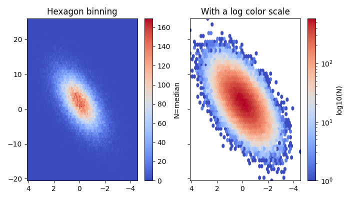
02. Point density with matplotlib.hexbin

This script demonstrates how to create a 2D hexagonal binning plot with matplotlib.hexbin. 🐝 This type of plot is an excellent alternative to a scatter plot for visualizing the density of a large number of points. The example generates random data and displays it using both linear and logarithmic color scales to represent point concentration.

Out:

C:\Users\kelda\Desktop\repositories\github\python-spare-code\main\examples\matplotlib\plot_main02_hexbin.py:59: UserWarning:

FigureCanvasAgg is non-interactive, and thus cannot be shown

import pandas as pd
import numpy as np
import matplotlib.pyplot as plt

# constant
n = 100000

# Fixing random state for reproducibility
np.random.seed(19680801)

# Generate data
x = np.random.standard_normal(n)
y = 2.0 + 3.0 * x + 4.0 * np.random.standard_normal(n)
z = None

# Compute limits
xmin = x.min()
xmax = x.max()
ymin = y.min()
ymax = y.max()

# Display hexagon binning (linear)
fig, axs = plt.subplots(ncols=2, sharey=True, figsize=(7, 4))
fig.subplots_adjust(hspace=0.5, left=0.07, right=0.93)
ax = axs[0]
hb = ax.hexbin(x, y, C=z, cmap='coolwarm', reduce_C_function=np.median)
ax.axis([xmin, xmax, ymin, ymax])
ax.set_title("Hexagon binning")
ax.invert_xaxis()
cb = fig.colorbar(hb, ax=ax)
cb.set_label('N=median')

# Display hexagon binning (log)
ax = axs[1]
hb = ax.hexbin(x, y, C=z, gridsize=50,
    bins='log', cmap='coolwarm',
    reduce_C_function=np.median)
ax.axis([xmin, xmax, ymin, ymax])
ax.set_title("With a log color scale")
ax.invert_xaxis()
cb = fig.colorbar(hb, ax=ax)
cb.set_label('log10(N)')

# Show
plt.tight_layout()
plt.show()