Note
Click here to download the full example code
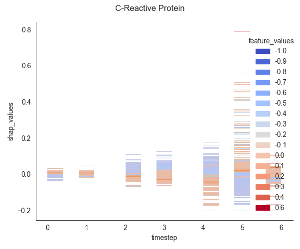
07.e 3D Data with sns.displot
Figure-level interface for drawing distribution plots onto a FacetGrid.
This script demonstrates how to use the figure-level function
seaborn.displot to create a 2D histogram where the bins are
colored by the values of a third, continuous variable. 🎨
- The core technique involves:
Plotting two variables on the x and y axes to show their joint distribution (in this case, timestep and shap_values).
Using the hue parameter to map a third variable (feature_values) to the color of each bin, effectively visualizing a third dimension on a 2D plot.
Leveraging Seaborn’s hue_norm to correctly scale the colormap to the range of the third variable.
Out:
          Unnamed: 0       sample     timestep  feature_values  shap_values
count    7000.000000  7000.000000  7000.000000     7000.000000  7000.000000
mean   126003.000000   499.500000     3.000000       -0.570943     0.000091
std     72751.329885   288.695612     2.000143        0.410149     0.042353
min        21.000000     0.000000     0.000000       -1.000000    -0.204305
25%     63012.000000   249.750000     1.000000       -0.900000    -0.011614
50%    126003.000000   499.500000     3.000000       -0.800000     0.000515
75%    188994.000000   749.250000     5.000000        0.000000     0.012057
max    251985.000000   999.000000     6.000000        0.600000     0.789859
 0. Computing... C-Reactive Protein
C:\Users\kelda\Desktop\repositories\github\python-spare-code\main\examples\matplotlib\plot_main07_e_displot.py:155: UserWarning:

FigureCanvasAgg is non-interactive, and thus cannot be shown
 22 import pandas as pd
 23 import seaborn as sns
 24 import matplotlib as mpl
 25 import matplotlib.pyplot as plt
 26
 27 from pathlib import Path
 28
 29 sns.set_style(style="white")
 30
 31
 32 def scalar_colormap(values, cmap, vmin, vmax):
 33     """This method creates a colormap based on values.
 34
 35     Parameters
 36     ----------
 37     values : array-like
 38     The values to create the corresponding colors
 39
 40     cmap : str
 41     The colormap
 42
 43     vmin, vmax : float
 44     The minimum and maximum possible values
 45
 46     Returns
 47     -------
 48     scalar colormap
 49     """
 50     # Create scalar mappable
 51     norm = mpl.colors.Normalize(vmin=vmin, vmax=vmax, clip=True)
 52     mapper = mpl.cm.ScalarMappable(norm=norm, cmap=cmap)
 53     # Get color map
 54     colormap = sns.color_palette([mapper.to_rgba(i) for i in values])
 55     # Return
 56     return colormap, norm
 57
 58 def scalar_palette(values, cmap, vmin, vmax):
 59     """This method creates a colorpalette based on values.
 60
 61     Parameters
 62     ----------
 63     values : array-like
 64     The values to create the corresponding colors
 65
 66     cmap : str
 67     The colormap
 68
 69     vmin, vmax : float
 70     The minimum and maximum possible values
 71
 72     Returns
 73     -------
 74     scalar colormap
 75
 76     """
 77     # Create a matplotlib colormap from name
 78     # cmap = sns.light_palette(cmap, reverse=False, as_cmap=True)
 79     cmap = sns.color_palette(cmap, as_cmap=True)
 80     # Normalize to the range of possible values from df["c"]
 81     norm = mpl.colors.Normalize(vmin=vmin, vmax=vmax)
 82     # Create a color dictionary (value in c : color from colormap)
 83     colors = {}
 84     for cval in values:
 85         colors.update({cval: cmap(norm(cval))})
 86     # Return
 87     return colors, norm
 88
 89
 90 # Load dataset
 91 path = Path('../../datasets/shap')
 92 data = pd.read_csv(path / 'shap.csv')
 93 data = data[data.features.isin(['C-Reactive Protein'])]
 94
 95 # Since the colorbar is discrete, needs to round so that
 96 # the amount of bins is small and therefore visible. Would
 97 # it be possible to define a continuous colormap?
 98 data.feature_values = data.feature_values.round(1)
 99
100 # Show
101 print(data.describe())
102
103 # Configuration
104 cmap_name = 'coolwarm' # colormap name
105
106
107 # .. note:: The function displot calls the histplot function. However,
108 #           the features allowed are count, frequency, probability or
109 #           proportion, percent and density. Thus, the median cannot
110 #           be computed.
111
112 # .. note:: The resulting colormap is discrete. Could it be continuous?
113
114 # Loop
115 for i, (name, df) in enumerate(data.groupby('features')):
116
117     # Info
118     print("%2d. Computing... %s" % (i, name))
119
120     # Get colormap
121     values = df.feature_values
122     cmap, norm = scalar_colormap(values=values,
123         cmap=cmap_name, vmin=values.min(),
124         vmax=values.max())
125
126     # Display displot
127     sns.displot(data=df, x='timestep', y='shap_values',
128         hue='feature_values', palette='coolwarm',
129         hue_norm=(values.min(), values.max()),
130         rug=False) # bins
131
132     """
133     # Display histplot
134     plt.figure()
135     sns.histplot(
136         data=df, x='timestep', y='shap_values',
137         discrete=(False, False),
138         hue='feature_values', palette=cmap_name,
139         hue_norm=(values.min(), values.max()),
140         cbar=False, cbar_kws=dict(shrink=.75),
141         #pthresh=.05, pmax=.9, bins=100
142     )
143     """
144
145     # Format figure
146     plt.suptitle(name)
147     plt.tight_layout()
148     plt.legend([], [], frameon=False)
149
150     # Show only first N
151     if int(i) > 2:
152         break
153
154 # Show
155 plt.show()
Total running time of the script: ( 0 minutes 2.860 seconds)