Note
Click here to download the full example code
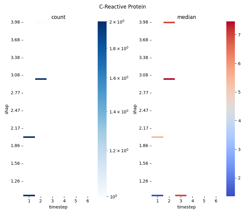
07.c stats.2dbin with fake data
This script provides a detailed example of how to aggregate 2D
point data into a grid and visualize it using seaborn.heatmap.
It uses simple, manually created data to clearly illustrate the
mechanics of the binning and plotting process.
The workflow includes:
Binning Data: It uses
scipy.stats.binned_statistic_2dto compute both the count of points and the median of values within each cell of a 2D grid.Advanced Heatmap Visualization: The resulting statistical matrices are plotted as two side-by-side heatmaps, demonstrating careful axis labeling, matrix flipping for correct orientation, and different color normalizations (LogNorm, robust scaling).
Out:
[1 1 1 1 2 2 2 3]
[1 1 2 2 3 3 4 1]
[1 1 5 6 7 8 7 7]

Scipy:
[0.5 1.5 2.5 3.5 4.5 5.5 6.5]
[1.         1.03030303 1.06060606 1.09090909 1.12121212 1.15151515
 1.18181818 1.21212121 1.24242424 1.27272727 1.3030303  1.33333333
 1.36363636 1.39393939 1.42424242 1.45454545 1.48484848 1.51515152
 1.54545455 1.57575758 1.60606061 1.63636364 1.66666667 1.6969697
 1.72727273 1.75757576 1.78787879 1.81818182 1.84848485 1.87878788
 1.90909091 1.93939394 1.96969697 2.         2.03030303 2.06060606
 2.09090909 2.12121212 2.15151515 2.18181818 2.21212121 2.24242424
 2.27272727 2.3030303  2.33333333 2.36363636 2.39393939 2.42424242
 2.45454545 2.48484848 2.51515152 2.54545455 2.57575758 2.60606061
 2.63636364 2.66666667 2.6969697  2.72727273 2.75757576 2.78787879
 2.81818182 2.84848485 2.87878788 2.90909091 2.93939394 2.96969697
 3.         3.03030303 3.06060606 3.09090909 3.12121212 3.15151515
 3.18181818 3.21212121 3.24242424 3.27272727 3.3030303  3.33333333
 3.36363636 3.39393939 3.42424242 3.45454545 3.48484848 3.51515152
 3.54545455 3.57575758 3.60606061 3.63636364 3.66666667 3.6969697
 3.72727273 3.75757576 3.78787879 3.81818182 3.84848485 3.87878788
 3.90909091 3.93939394 3.96969697 4.        ]
[[2. 0. 1. 0. 0. 0.]
 [0. 0. 0. 0. 0. 0.]
 [0. 0. 0. 0. 0. 0.]
 [0. 0. 0. 0. 0. 0.]
 [0. 0. 0. 0. 0. 0.]
 [0. 0. 0. 0. 0. 0.]
 [0. 0. 0. 0. 0. 0.]
 [0. 0. 0. 0. 0. 0.]
 [0. 0. 0. 0. 0. 0.]
 [0. 0. 0. 0. 0. 0.]
 [0. 0. 0. 0. 0. 0.]
 [0. 0. 0. 0. 0. 0.]
 [0. 0. 0. 0. 0. 0.]
 [0. 0. 0. 0. 0. 0.]
 [0. 0. 0. 0. 0. 0.]
 [0. 0. 0. 0. 0. 0.]
 [0. 0. 0. 0. 0. 0.]
 [0. 0. 0. 0. 0. 0.]
 [0. 0. 0. 0. 0. 0.]
 [0. 0. 0. 0. 0. 0.]
 [0. 0. 0. 0. 0. 0.]
 [0. 0. 0. 0. 0. 0.]
 [0. 0. 0. 0. 0. 0.]
 [0. 0. 0. 0. 0. 0.]
 [0. 0. 0. 0. 0. 0.]
 [0. 0. 0. 0. 0. 0.]
 [0. 0. 0. 0. 0. 0.]
 [0. 0. 0. 0. 0. 0.]
 [0. 0. 0. 0. 0. 0.]
 [0. 0. 0. 0. 0. 0.]
 [0. 0. 0. 0. 0. 0.]
 [0. 0. 0. 0. 0. 0.]
 [0. 0. 0. 0. 0. 0.]
 [2. 0. 0. 0. 0. 0.]
 [0. 0. 0. 0. 0. 0.]
 [0. 0. 0. 0. 0. 0.]
 [0. 0. 0. 0. 0. 0.]
 [0. 0. 0. 0. 0. 0.]
 [0. 0. 0. 0. 0. 0.]
 [0. 0. 0. 0. 0. 0.]
 [0. 0. 0. 0. 0. 0.]
 [0. 0. 0. 0. 0. 0.]
 [0. 0. 0. 0. 0. 0.]
 [0. 0. 0. 0. 0. 0.]
 [0. 0. 0. 0. 0. 0.]
 [0. 0. 0. 0. 0. 0.]
 [0. 0. 0. 0. 0. 0.]
 [0. 0. 0. 0. 0. 0.]
 [0. 0. 0. 0. 0. 0.]
 [0. 0. 0. 0. 0. 0.]
 [0. 0. 0. 0. 0. 0.]
 [0. 0. 0. 0. 0. 0.]
 [0. 0. 0. 0. 0. 0.]
 [0. 0. 0. 0. 0. 0.]
 [0. 0. 0. 0. 0. 0.]
 [0. 0. 0. 0. 0. 0.]
 [0. 0. 0. 0. 0. 0.]
 [0. 0. 0. 0. 0. 0.]
 [0. 0. 0. 0. 0. 0.]
 [0. 0. 0. 0. 0. 0.]
 [0. 0. 0. 0. 0. 0.]
 [0. 0. 0. 0. 0. 0.]
 [0. 0. 0. 0. 0. 0.]
 [0. 0. 0. 0. 0. 0.]
 [0. 0. 0. 0. 0. 0.]
 [0. 0. 0. 0. 0. 0.]
 [0. 2. 0. 0. 0. 0.]
 [0. 0. 0. 0. 0. 0.]
 [0. 0. 0. 0. 0. 0.]
 [0. 0. 0. 0. 0. 0.]
 [0. 0. 0. 0. 0. 0.]
 [0. 0. 0. 0. 0. 0.]
 [0. 0. 0. 0. 0. 0.]
 [0. 0. 0. 0. 0. 0.]
 [0. 0. 0. 0. 0. 0.]
 [0. 0. 0. 0. 0. 0.]
 [0. 0. 0. 0. 0. 0.]
 [0. 0. 0. 0. 0. 0.]
 [0. 0. 0. 0. 0. 0.]
 [0. 0. 0. 0. 0. 0.]
 [0. 0. 0. 0. 0. 0.]
 [0. 0. 0. 0. 0. 0.]
 [0. 0. 0. 0. 0. 0.]
 [0. 0. 0. 0. 0. 0.]
 [0. 0. 0. 0. 0. 0.]
 [0. 0. 0. 0. 0. 0.]
 [0. 0. 0. 0. 0. 0.]
 [0. 0. 0. 0. 0. 0.]
 [0. 0. 0. 0. 0. 0.]
 [0. 0. 0. 0. 0. 0.]
 [0. 0. 0. 0. 0. 0.]
 [0. 0. 0. 0. 0. 0.]
 [0. 0. 0. 0. 0. 0.]
 [0. 0. 0. 0. 0. 0.]
 [0. 0. 0. 0. 0. 0.]
 [0. 0. 0. 0. 0. 0.]
 [0. 0. 0. 0. 0. 0.]
 [0. 0. 0. 0. 0. 0.]
 [0. 1. 0. 0. 0. 0.]]
[1.01515152 1.04545455 1.07575758 1.10606061 1.13636364 1.16666667
 1.1969697  1.22727273 1.25757576 1.28787879 1.31818182 1.34848485
 1.37878788 1.40909091 1.43939394 1.46969697 1.5        1.53030303
 1.56060606 1.59090909 1.62121212 1.65151515 1.68181818 1.71212121
 1.74242424 1.77272727 1.8030303  1.83333333 1.86363636 1.89393939
 1.92424242 1.95454545 1.98484848 2.01515152 2.04545455 2.07575758
 2.10606061 2.13636364 2.16666667 2.1969697  2.22727273 2.25757576
 2.28787879 2.31818182 2.34848485 2.37878788 2.40909091 2.43939394
 2.46969697 2.5        2.53030303 2.56060606 2.59090909 2.62121212
 2.65151515 2.68181818 2.71212121 2.74242424 2.77272727 2.8030303
 2.83333333 2.86363636 2.89393939 2.92424242 2.95454545 2.98484848
 3.01515152 3.04545455 3.07575758 3.10606061 3.13636364 3.16666667
 3.1969697  3.22727273 3.25757576 3.28787879 3.31818182 3.34848485
 3.37878788 3.40909091 3.43939394 3.46969697 3.5        3.53030303
 3.56060606 3.59090909 3.62121212 3.65151515 3.68181818 3.71212121
 3.74242424 3.77272727 3.8030303  3.83333333 3.86363636 3.89393939
 3.92424242 3.95454545 3.98484848]
[1. 2. 3. 4. 5. 6.]
C:\Users\kelda\Desktop\repositories\github\python-spare-code\main\examples\matplotlib\plot_main07_c_2dbin_fake.py:164: UserWarning:

FigureCanvasAgg is non-interactive, and thus cannot be shown


'\nimport sys\nsys.exit()\n# Compute bin statistic (count and median)\n\n# Plot\nplt.figure()\nsns.violinplot(data=data, x="timestep", y="shap_values", inner="box")\nplt.figure()\nplt.tight_layout()\nsns.violinplot(data=data, x="timestep", y="feature_values", inner="box")\nplt.figure()\nsns.histplot(data=data, x="timestep", shrink=.8)\n\n\n# Plot hist\nf1 = plt.hist2d(data.timestep, data.feature_values, bins=30, cmap=\'Reds\')\ncb = plt.colorbar()\ncb.set_label(\'counts in bin\')\nplt.title(\'Counts (square bin)\')\nplt.show()\n'
 22 # Libraries
 23 import seaborn as sns
 24 import pandas as pd
 25 import numpy as np
 26 import matplotlib.pyplot as plt
 27
 28 from scipy import stats
 29 from matplotlib.colors import LogNorm
 30
 31 def data_shap():
 32     data = pd.read_csv('../../datasets/shap/shap.csv')
 33     return data.timestep, \
 34            data.shap_values, \
 35            data.feature_values, \
 36            data
 37
 38 def data_manual():
 39     """"""
 40     # Create random values
 41     x = np.array([1, 1, 1, 1, 2, 2, 2, 3])
 42     y = np.array([1, 1, 2, 2, 3, 3, 4, 1])
 43     z = np.array([1, 1, 5, 6, 7, 8, 7, 7])
 44     return x, y, z, None
 45
 46 # Create data
 47 x, y, z, data = data_manual()
 48
 49 print(x)
 50 print(y)
 51 print(z)
 52
 53 """
 54 # With pandas
 55 v = z
 56 vals, bins = np.histogram(v)
 57 a = pd.Series(v).groupby(pd.cut(v, bins)).median()
 58 print("\nPandas:")
 59 print(bins)
 60 print(vals)
 61 print(a)
 62 """
 63
 64
 65
 66
 67
 68
 69
 70 vmin = z.min()
 71 vmax = z.max()
 72
 73
 74
 75 # Compute binned statistic (median)
 76 binx = np.linspace(0, 3, 4) + 0.5
 77 biny = np.linspace(0, 4, 5) + 0.5
 78 binx = np.linspace(0, 6, 7) + 0.5
 79 biny = np.linspace(y.min(), y.max(), 100)
 80 r1 = stats.binned_statistic_2d(x=y, y=x, values=z,
 81     statistic='count', bins=[biny, binx],
 82     expand_binnumbers=False)
 83
 84 r2 = stats.binned_statistic_2d(x=y, y=x, values=z,
 85     statistic='median', bins=[biny, binx],
 86     expand_binnumbers=False)
 87
 88 # Compute centres
 89 x_center = (r1.x_edge[:-1] + r1.x_edge[1:]) / 2
 90 y_center = (r1.y_edge[:-1] + r1.y_edge[1:]) / 2
 91
 92 # Show
 93 print("\nScipy:")
 94 print(binx)
 95 print(biny)
 96 print(r1.statistic)
 97 print(x_center)
 98 print(y_center)
 99
100 # Convert the computed matrix to an stacked dataframe?
101
102 flip1 = np.flip(r1.statistic, 0)
103 flip2 = np.flip(r2.statistic, 0)
104 #flip1 = r1.statistic
105 #flip2 = r2.statistic
106
107
108
109 # Display
110 fig, axs = plt.subplots(nrows=1, ncols=2,
111     sharey=False, sharex=False, figsize=(8, 7))
112
113 sns.heatmap(flip1, annot=False, linewidth=0.5,
114     xticklabels=y_center.astype(int),
115     yticklabels=x_center.round(2)[::-1], # Because of flip
116     cmap='Blues', ax=axs[0],
117     norm=LogNorm())
118
119 sns.heatmap(flip2, annot=False, linewidth=0.5,
120     xticklabels=y_center.astype(int),
121     yticklabels=x_center.round(2)[::-1], # Because of flip
122     cmap='coolwarm', ax=axs[1], zorder=1,
123     vmin=None, vmax=None, center=None, robust=True)
124
125 # If robust=True and vmin or vmax are absent, the colormap range
126 # is computed with robust quantiles instead of the extreme values.
127 """
128 sns.violinplot(x=x, y=y,
129     saturation=0.5, fliersize=0.1, linewidth=0.5,
130     color='green', ax=axs[2], zorder=3,
131     width=0.5)
132 """
133
134
135 # Configure ax0
136 axs[0].set_title('count')
137 axs[0].set_xlabel('timestep')
138 axs[0].set_ylabel('shap')
139 axs[0].locator_params(axis='y', nbins=10)
140 #axs[0].set_aspect('equal', 'box'
141
142 # Configure ax1
143 axs[1].set_title('median')
144 axs[1].set_xlabel('timestep')
145 axs[1].set_ylabel('shap')
146 axs[1].locator_params(axis='y', nbins=10)
147 #axs[1].set_aspect('equal', 'box')
148 #axs[1].invert_yaxis()
149
150 # Generic
151 plt.suptitle('C-Reactive Protein')
152
153 """
154 # Set axes manually
155 #plt.set_xticks()
156 #plt.setp(axs[1].get_yticklabels()[::1], visible=False)
157 #plt.setp(axs[1].get_yticklabels()[::5], visible=True)
158 from matplotlib import ticker
159 axs[1].xaxis.set_major_locator(ticker.MultipleLocator(1.00))
160 axs[1].xaxis.set_minor_locator(ticker.MultipleLocator(0.25))
161 """
162
163 plt.tight_layout()
164 plt.show()
165
166
167 """
168 import sys
169 sys.exit()
170 # Compute bin statistic (count and median)
171
172 # Plot
173 plt.figure()
174 sns.violinplot(data=data, x="timestep", y="shap_values", inner="box")
175 plt.figure()
176 plt.tight_layout()
177 sns.violinplot(data=data, x="timestep", y="feature_values", inner="box")
178 plt.figure()
179 sns.histplot(data=data, x="timestep", shrink=.8)
180
181
182 # Plot hist
183 f1 = plt.hist2d(data.timestep, data.feature_values, bins=30, cmap='Reds')
184 cb = plt.colorbar()
185 cb.set_label('counts in bin')
186 plt.title('Counts (square bin)')
187 plt.show()
188 """
Total running time of the script: ( 0 minutes 1.063 seconds)