0.4 Visualizing GMM and KDE

This script demonstrates and contrasts two common density estimation techniques on synthetic, clustered data.

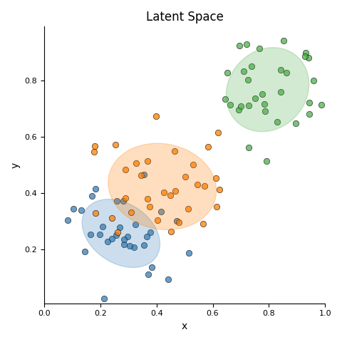
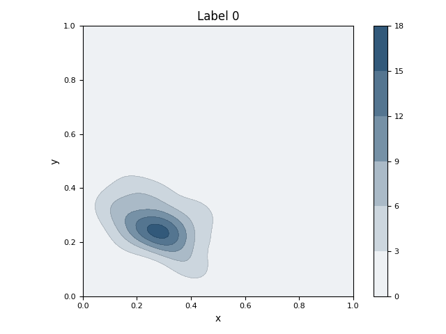
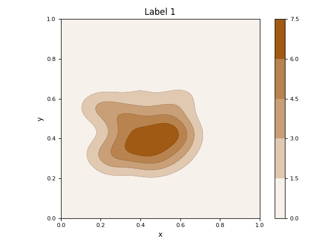
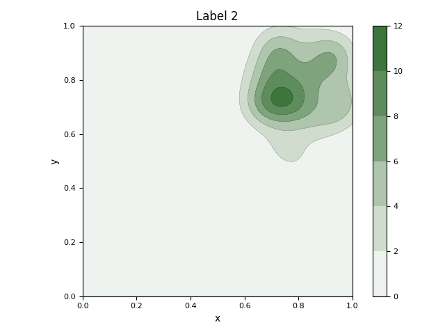
This script first generates a synthetic 2D dataset with three distinct clusters using sklearn.datasets.make_blobs. It then fits a Gaussian Mixture Model (GMM) to the entire dataset to parametrically model the underlying distributions of the clusters. The initial visualization displays the raw data points as a scatter plot, with ellipses overlaid to represent the mean and covariance of each learned Gaussian component. Subsequently, the script isolates the data for each class and calculates its non-parametric Kernel Density Estimation (KDE). It generates a separate contour plot for each class, visually representing the probability density of the data points within that specific group.

Note

https://jakevdp.github.io/PythonDataScienceHandbook/04.05-histograms-and-binnings.html

• 
• 
• 
• 

Out:

Ignoring fixed y limits to fulfill fixed data aspect with adjustable data limits.
C:\Users\kelda\Desktop\repositories\github\python-spare-code\main\examples\matplotlib\plot_main04_gmm_kde.py:334: UserWarning: FigureCanvasAgg is non-interactive, and thus cannot be shown

# Libraries
import numpy as np
import pandas as pd
import matplotlib as mpl
import matplotlib.pyplot as plt

# Specific
from scipy import linalg
from sklearn import mixture
from sklearn.datasets import make_blobs
from sklearn.preprocessing import MinMaxScaler
from scipy.stats import gaussian_kde
from matplotlib.colors import LinearSegmentedColormap

# Latexify
mpl.rc('font', size=10)
mpl.rc('legend', fontsize=6)
mpl.rc('xtick', labelsize=8)
mpl.rc('ytick', labelsize=8)


# -----------------------------------------
# Methods
# -----------------------------------------
def make_colormap(seq):
    """Return a LinearSegmentedColormap

    Parameters
    ----------
    seq: list
        A sequence of floats and RGB-tuples. The floats
        should be increasing and in the interval (0,1).
    """
    # Library
    import matplotlib.colors as mcolors
    # Code
    seq = [(None,) * 3, 0.0] + list(seq) + [1.0, (None,) * 3]
    cdict = {'red': [], 'green': [], 'blue': []}
    for i, item in enumerate(seq):
        if isinstance(item, float):
            r1, g1, b1 = seq[i - 1]
            r2, g2, b2 = seq[i + 1]
            cdict['red'].append([item, r1, r2])
            cdict['green'].append([item, g1, g2])
            cdict['blue'].append([item, b1, b2])
    return mcolors.LinearSegmentedColormap('CustomMap', cdict)

def adjust_lightness(color, amount=0.5):
    """Adjusts the lightness of a color

    Parameters
    ----------
    color: string or vector
        The color in string, hex or rgb format.

    amount: float
        Lower values result in dark colors.
    """
    # Libraries
    import matplotlib.colors as mc
    import colorsys
    try:
        c = mc.cnames[color]
    except:
        c = color
    c = colorsys.rgb_to_hls(*mc.to_rgb(c))
    return colorsys.hls_to_rgb(c[0], \
        max(0, min(1, amount * c[1])), c[2])

def kde_mpl_compute(x, y, xlim=None, ylim=None, **kwargs):
    """Computes the gaussian kde.

    Parameters
    ----------

    Returns
    -------
    """
    try:
        # Plot density
        kde = gaussian_kde(np.vstack((x, y)), **kwargs)
    except Exception as e:
        print("Exception! %s" % e)
        return None, None, None

    # Parameters
    xmin, xmax = min(x), max(x)
    ymin, ymax = min(y), max(y)

    # Set xlim and ylim
    if xlim is not None:
        xmin, xmax = xlim
    if ylim is not None:
        ymin, ymax = ylim

    # evaluate on a regular grid
    xgrid = np.linspace(xmin, xmax, 100)
    ygrid = np.linspace(ymin, ymax, 100)
    Xgrid, Ygrid = np.meshgrid(xgrid, ygrid)
    zgrid = kde.evaluate(np.vstack([
        Xgrid.ravel(),
        Ygrid.ravel()
    ]))
    Zgrid = zgrid.reshape(Xgrid.shape)

    # Return
    return xgrid, ygrid, Zgrid

def plot_ellipses(gmm, ax, color, n=None):
    """Plot ellipses from GaussianMixtureModel"""

    # Define color
    if color is None:
        color = 'blue'
    if n is None:
        n = 1

    # Get covariances
    if gmm.covariance_type == 'full':
        covariances = gmm.covariances_[n][:2, :2]
    elif gmm.covariance_type == 'tied':
        covariances = gmm.covariances_[:2, :2]
    elif gmm.covariance_type == 'diag':
        covariances = np.diag(gmm.covariances_[n][:2])
    elif gmm.covariance_type == 'spherical':
        covariances = np.eye(gmm.means_.shape[1]) * gmm.covariances_[n]

    # Compute
    v, w = np.linalg.eigh(covariances)
    # v = 2. * np.sqrt(2.) * np.sqrt(v) # Oliver
    u = w[0] / np.linalg.norm(w[0])
    angle = np.arctan2(u[1], u[0])
    angle = 180 * angle / np.pi  # convert to degrees
    v = 2. * np.sqrt(2.) * np.sqrt(v)

    # Plot
    ell = mpl.patches.Ellipse(gmm.means_[n, :2],
        v[0], v[1], angle=180 + angle, color=color)
    ell.set_clip_box(ax.bbox)
    ell.set_alpha(0.25)
    ax.add_artist(ell)
    ax.set_aspect('equal', 'datalim')


# -----------------------------------------
# Create data
# -----------------------------------------
# Colors
colors = ['#377eb8', '#ff7f00', '#4daf4a',
          '#a65628', '#984ea3',
          '#999999', '#e41a1c', '#dede00']

c1 = colors[0]
c2 = colors[1]
c3 = colors[2]

# Data
data = [
    [0.19, 0.25, 0, 1, 0, 0, 0],
    [0.15, 0.21, 0, 1, 0, 0, 0],
    [0.13, 0.19, 0, 1, 0, 0, 0],
    [0.16, 0.12, 0, 1, 0, 0, 0],
    [0.21, 0.14, 0, 1, 0, 0, 0],
    [0.38, 0.18, 0, 1, 0, 0, 0],

    [0.50, 0.52, 1, 0, 1, 0, 0],
    [0.40, 0.58, 1, 0, 1, 0, 0],
    [0.49, 0.72, 1, 0, 1, 0, 0],
    [0.44, 0.64, 1, 0, 1, 0, 0],
    [0.60, 0.50, 1, 0, 1, 0, 0],
    [0.38, 0.81, 1, 0, 1, 0, 0],
    [0.40, 0.75, 1, 0, 1, 0, 0],
    [0.47, 0.61, 1, 0, 1, 0, 0],
    [0.52, 0.65, 1, 0, 1, 0, 0],
    [0.50, 0.55, 1, 0, 1, 0, 0],
    [0.46, 0.54, 1, 0, 1, 0, 0],
    [0.60, 0.50, 1, 0, 1, 0, 0],
    [0.68, 0.52, 1, 0, 1, 0, 0],
    [0.61, 0.77, 1, 0, 1, 0, 0],
    [0.51, 0.79, 1, 0, 1, 0, 1],
    [0.64, 0.80, 1, 0, 1, 0, 1],
    [0.54, 0.75, 1, 0, 1, 0, 1],
    [0.58, 0.81, 1, 0, 1, 0, 1],

    [0.80, 0.82, 2, 0, 0, 1, 1],
    [0.85, 0.83, 2, 0, 0, 1, 1],
    [0.90, 0.85, 2, 0, 0, 1, 1],
    [0.84, 0.80, 2, 0, 0, 1, 1],
    [0.81, 0.78, 2, 0, 0, 1, 1],
    [0.92, 0.79, 2, 0, 0, 1, 1],
]

"""
# Create DataFrame (manual data)
data = pd.DataFrame(data)
data.columns = ['x', 'y', 'target',
    'Label 0', 'Label 1', 'Label 2',
    'Label 3']
"""

# Create bloobs
X, y = make_blobs(n_features=2,
    centers=[[0.35, 0.35],
             [0.45, 0.45],
             [0.7, 0.70]],
    cluster_std=[0.07, 0.10, 0.07])

# Preprocessing
X = MinMaxScaler().fit_transform(X)

# Create Dataframe
data = pd.DataFrame(X, columns=['x', 'y'])
data['target'] = y
for i in np.unique(y):
    data['Label %s' % i] = y==i
data = data[(data.x>0) & (data.x<1)]
data = data[(data.y>0) & (data.y<1)]

# Create X
X = data[['x', 'y']]

# Create gaussian
gmm = mixture.GaussianMixture(
    n_components=3, covariance_type='full')

# Since we have class labels for the training data, we can
# initialize the GMM parameters in a supervised manner.
gmm.means_init = np.array( \
    [X[data.target == i].mean(axis=0)
        for i in range(3)])

# Fit a Gaussian mixture with EM using five components
gmm = gmm.fit(data[['x', 'y']])


# -----------------------------------------
# Visualisation (
# -----------------------------------------
# Create figure
figure, ax = plt.subplots(1,1, figsize=(4.8, 4.8))

for i, (c, aux) in enumerate(data.groupby('target')):

    # Plot markers
    ax.scatter(aux.x, aux.y, c=colors[i],
       edgecolors='k', alpha=0.75,
       linewidths=0.5)

    # Plot ellipse
    plot_ellipses(gmm, ax, color=colors[i], n=i)

# Configure
ax.set(xlabel='x', ylabel='y',
       aspect='equal',
       xlim=[0, 1], ylim=[0, 1],
       title='Latent Space')

# Hide the right and top spines
ax.spines.right.set_visible(False)
ax.spines.top.set_visible(False)

# Adjust
plt.tight_layout()


# -----------------------------------------
# Visualisation labels
# -----------------------------------------
# Loop
for i, l in enumerate(['Label 0',
                       'Label 1',
                       'Label 2']):
    # Filter data
    aux = data[data[l] == 1]

    # Compute KDE
    xgrid, ygrid, Zgrid = \
        kde_mpl_compute(aux.x, aux.y,
            xlim=[0, 1], ylim=[0, 1])

    # Create colormap
    cmap = LinearSegmentedColormap.from_list("",
         ['white', adjust_lightness(colors[i], 0.6)], 14)

    # Create figure
    figure, ax = plt.subplots(1,1)

    # Plot contour
    ax.contour(xgrid, ygrid, Zgrid,
       linewidths=0.25, alpha=0.5, levels=5,
       linestyles='dashed', colors='k')
    # Plot fill spaces
    cntr = ax.contourf(xgrid, ygrid, Zgrid,
       levels=5, cmap=cmap)
    # Add colorbar
    cb = plt.colorbar(cntr, ax=ax)

    # Configure
    ax.set(xlabel='x', ylabel='y',
           aspect='equal', title=l,
           xlim=[0, 1], ylim=[0, 1])

    # Adjust
    plt.tight_layout()


# -----------------------------------------
# All together
# -----------------------------------------

# Con
plt.show()