Note
Go to the end to download the full example code
SARI - Compute timeseries
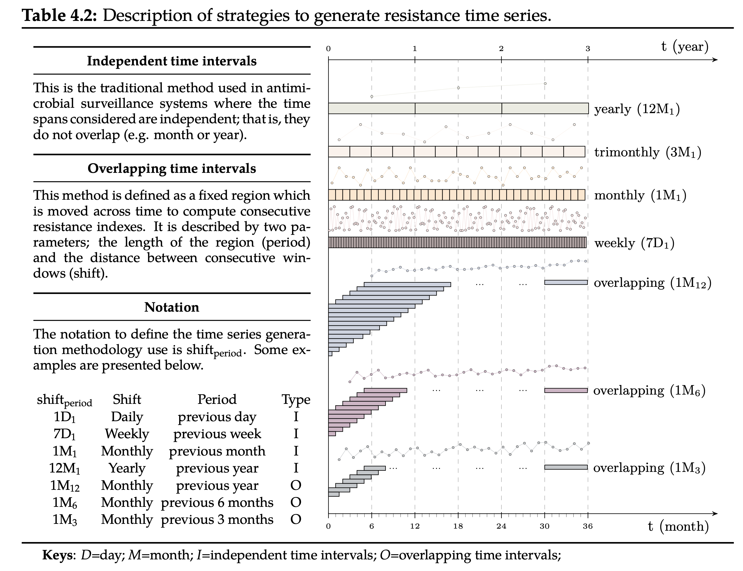
In order to study the temporal evolution of AMR, it is necessary to generate a resistance time series from the susceptibility test data. This is often achieved by computing the resistance index on consecutive partitions of the data. Note that each partition contains the susceptibility tests required to compute a resistance index. The traditional strategy of dealing with partitions considers independent time intervals (see yearly, monthly or weekly time series in Table 4.2). Unfortunately, this strategy forces to trade-off between granularity (level of detail) and accuracy. On one side, weekly time series are highly granular but inaccurate. On the other hand, yearly time series are accurate but rough. Note that the granularity is represented by the number of observations in a time series while the accuracy is closely related with the number of susceptibility tests used to compute the resistance index. Conversely, the overlapping time intervals strategy drops such dependence by defining a window of fixed size which is moved across time. The length of the window is denoted as period and the time step as shift. For instance, three time series obtained using the overlapping time intervals strategy with a monthly shift (1M) and window lengths of 12, 6 and 3 have been presented for the sake of clarity (see 1M12, 1M6 and 1M3 in Table 4.2).

The notation to define the time series generation methodology (SHIFTperiod) is described with various examples in Table 4.2. For instance, 7D4 defines a time series with weekly resistance indexes (7D) calculated using the microbiology records available for the previous four weeks (4x7D). It is important to note that some notations are equivalent representations of the same susceptibility data at different granularities, hence their trends are comparable. As an example, the trend estimated for 1M1 should be approximately thirty times the trend estimated for 1D30.
Let’s see how to compute SARI time series with examples.
We first load the data and select one single pair for clarity.
 53 # Libraries
 54 import numpy as np
 55 import pandas as pd
 56 import seaborn as sns
 57 import matplotlib as mpl
 58 import matplotlib.pyplot as plt
 59
 60 # Import own libraries
 61 from pyamr.core.sari import sari
 62 from pyamr.datasets.load import load_data_nhs
 63
 64 # -------------------------
 65 # Configuration
 66 # -------------------------
 67 # Configure seaborn style (context=talk)
 68 sns.set(style="white")
 69
 70 # Set matplotlib
 71 mpl.rcParams['xtick.labelsize'] = 9
 72 mpl.rcParams['ytick.labelsize'] = 9
 73 mpl.rcParams['axes.titlesize'] = 11
 74 mpl.rcParams['legend.fontsize'] = 9
 75
 76 # Pandas configuration
 77 pd.set_option('display.max_colwidth', 40)
 78 pd.set_option('display.width', 300)
 79 pd.set_option('display.precision', 4)
 80
 81 # Numpy configuration
 82 np.set_printoptions(precision=2)
 83
 84 # -------------------------------------------
 85 # Load data
 86 # -------------------------------------------
 87 # Load data
 88 data, antimicrobials, microorganisms = load_data_nhs()
 89
 90 # Show
 91 print("\nData:")
 92 print(data)
 93 print("\nColumns:")
 94 print(data.columns)
 95 print("\nDtypes:")
 96 print(data.dtypes)
 97
 98 # Filter
 99 idxs_spec = data.specimen_code.isin(['URICUL'])
100 idxs_orgs = data.microorganism_code.isin(['ECOL'])
101 idxs_abxs = data.antimicrobial_code.isin(['AAUG'])
102
103 # Filter
104 data = data[idxs_spec & idxs_orgs & idxs_abxs]
105
106 # Filter dates (2016-2018 missing)
107 data = data[data.date_received.between('2008-01-01', '2016-12-31')]
Data:
           date_received         date_outcome patient_id laboratory_number specimen_code                   specimen_name  ... antimicrobial_code       antimicrobial_name sensitivity_method sensitivity  mic reported
0    2009-01-03 00:00:00                  NaN      20091           X428501        BLDCUL                             NaN  ...               AAMI                 amikacin                NaN   sensitive  NaN      NaN
1    2009-01-03 00:00:00                  NaN      20091           X428501        BLDCUL                             NaN  ...               AAMO              amoxycillin                NaN   resistant  NaN      NaN
2    2009-01-03 00:00:00                  NaN      20091           X428501        BLDCUL                             NaN  ...               AAUG                augmentin                NaN   sensitive  NaN      NaN
3    2009-01-03 00:00:00                  NaN      20091           X428501        BLDCUL                             NaN  ...               AAZT                aztreonam                NaN   sensitive  NaN      NaN
4    2009-01-03 00:00:00                  NaN      20091           X428501        BLDCUL                             NaN  ...               ACAZ              ceftazidime                NaN   sensitive  NaN      NaN
...                  ...                  ...        ...               ...           ...                             ...  ...                ...                      ...                ...         ...  ...      ...
7929 2021-01-21 23:56:00  2021-01-22 00:00:00     199863          H2230229         FBCUL  Fluid in Blood Culture Bottles  ...               AGEN               gentamicin                 DD   resistant  NaN        Y
7930 2021-01-21 23:56:00  2021-01-22 00:00:00     199863          H2230229         FBCUL  Fluid in Blood Culture Bottles  ...               AMER                meropenem                 DD   sensitive  NaN        Y
7931 2021-01-21 23:56:00  2021-01-22 00:00:00     199863          H2230229         FBCUL  Fluid in Blood Culture Bottles  ...               ATAZ  piperacillin-tazobactam                 DD   sensitive  NaN        N
7932 2021-01-21 23:56:00  2021-01-22 00:00:00     199863          H2230229         FBCUL  Fluid in Blood Culture Bottles  ...               ATEM               temocillin                 DD   sensitive  NaN        N
7933 2021-01-21 23:56:00  2021-01-22 00:00:00     199863          H2230229         FBCUL  Fluid in Blood Culture Bottles  ...               ATIG              tigecycline                 DD   sensitive  NaN        N

[3770034 rows x 15 columns]

Columns:
Index(['date_received', 'date_outcome', 'patient_id', 'laboratory_number', 'specimen_code', 'specimen_name', 'specimen_description', 'microorganism_code', 'microorganism_name', 'antimicrobial_code', 'antimicrobial_name', 'sensitivity_method', 'sensitivity', 'mic', 'reported'], dtype='object')

Dtypes:
date_received           datetime64[ns]
date_outcome                    object
patient_id                      object
laboratory_number               object
specimen_code                   object
specimen_name                   object
specimen_description            object
microorganism_code              object
microorganism_name              object
antimicrobial_code              object
antimicrobial_name              object
sensitivity_method              object
sensitivity                     object
mic                             object
reported                        object
dtype: object
Independent Time Intervals (ITI)
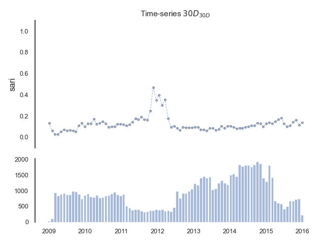
This is the traditional method used in antimicrobial surveillance systems where the time spans considered are independent; that is, they do not overlap (e.g. monthly time series - 1M1 or yearly timeseries - 12M1).
118 # -------------------------------------------
119 # Compute ITI sari (temporal)
120 # -------------------------------------------
121 from pyamr.core.sari import SARI
122
123 # Create SARI instance
124 sar = SARI(groupby=['specimen_code',
125                      'microorganism_code',
126                      'antimicrobial_code',
127                      'sensitivity'])
128
129 # Create constants
130 shift, period = '30D', '30D'
131
132 # Compute sari timeseries
133 iti = sar.compute(data, shift=shift,
134     period=period, cdate='date_received')
135
136 # Reset index
137 iti = iti.reset_index()
138
139
140 # --------------
141 # Plot
142 # --------------
143 # Create figure
144 fig, axes = plt.subplots(2, 1, sharex=True,
145         gridspec_kw={'height_ratios': [2, 1]})
146 axes = axes.flatten()
147
148 # Plot line
149 sns.lineplot(x=iti.date_received, y=iti.sari,
150     palette="tab10", linewidth=0.75, linestyle='--',
151     marker='o', markersize=3, markeredgecolor='k',
152     markeredgewidth=0.5, markerfacecolor=None,
153     alpha=0.5, ax=axes[0])
154
155 # Compute widths
156 widths = [d.days for d in np.diff(iti.date_received.tolist())]
157
158 # Plot bars
159 axes[1].bar(x=iti.date_received, height=iti.freq,
160     width=.8*widths[0], linewidth=0.75, alpha=0.5)
161
162 # Configure
163 axes[0].set(ylim=[-0.1, 1.1],
164     title='Time-series $%s_{%s}$' % (shift, period))
165
166 # Despine
167 sns.despine(bottom=True)
168
169 # Tight layout
170 plt.tight_layout()
171
172 # Show
173 print("\nTemporal (ITI):")
174 print(iti)

Temporal (ITI):
   specimen_code microorganism_code antimicrobial_code date_received  intermediate  resistant  sensitive   freq    sari
0         URICUL               ECOL               AAUG    2009-01-03           0.0        5.0       32.0   37.0  0.1351
1         URICUL               ECOL               AAUG    2009-02-02           0.0        7.0      107.0  114.0  0.0614
2         URICUL               ECOL               AAUG    2009-03-04           0.0       26.0      904.0  930.0  0.0280
3         URICUL               ECOL               AAUG    2009-04-03           0.0       23.0      812.0  835.0  0.0275
4         URICUL               ECOL               AAUG    2009-05-03           0.0       48.0      839.0  887.0  0.0541
..           ...                ...                ...           ...           ...        ...        ...    ...     ...
81        URICUL               ECOL               AAUG    2015-08-30           3.0       72.0      606.0  681.0  0.1101
82        URICUL               ECOL               AAUG    2015-09-29           0.0       97.0      586.0  683.0  0.1420
83        URICUL               ECOL               AAUG    2015-10-29           2.0      117.0      606.0  725.0  0.1641
84        URICUL               ECOL               AAUG    2015-11-28           0.0       85.0      658.0  743.0  0.1144
85        URICUL               ECOL               AAUG    2015-12-28           0.0       32.0      196.0  228.0  0.1404

[86 rows x 9 columns]
Overlapping Time Intervals (OTI)
This method is defined as a fixed region which is moved across time to compute consecutive
resistance indexes. It is described by two parameters SHIFTperiod where period denotes the
length of the window and shift the distance between consecutive windows. This approach
it is more versatile and allows to include larger number of susceptibility tests when
computing sari. Therefore, this is useful in scenarios in which pairs do
not have a large number of records in the dataset.
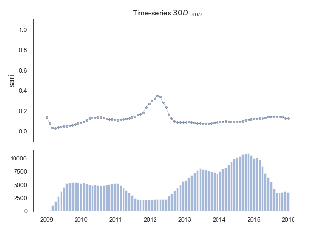
Note how the sari values are now larger than in the previous example!!
191 # -------------------------------------------
192 # Compute OTI sari (temporal)
193 # -------------------------------------------
194 # Variables
195 shift, period = '30D', '180D'
196
197 # Compute sari timeseries
198 oti = sar.compute(data, shift=shift,
199     period=period, cdate='date_received')
200
201 # Reset index
202 oti = oti.reset_index()
203
204 # --------------
205 # Plot
206 # --------------
207 # Create figure
208 fig, axes = plt.subplots(2, 1, sharex=True,
209         gridspec_kw={'height_ratios': [2, 1]})
210 axes = axes.flatten()
211
212 # Plot line
213 sns.lineplot(x=oti.date_received, y=oti.sari,
214     palette="tab10", linewidth=0.75, linestyle='--',
215     marker='o', markersize=3, markeredgecolor='k',
216     markeredgewidth=0.5, markerfacecolor=None,
217     alpha=0.5, ax=axes[0])
218
219 # Compute widths
220 widths = [d.days for d in np.diff(oti.date_received.tolist())]
221
222 # Plot bars
223 axes[1].bar(x=oti.date_received, height=oti.freq,
224     width=.8*widths[0], linewidth=0.75, alpha=0.5)
225
226 # Configure
227 axes[0].set(ylim=[-0.1, 1.1],
228     title='Time-series $%s_{%s}$' % (shift, period))
229
230 # Despine
231 sns.despine(bottom=True)
232
233 # Tight layout
234 plt.tight_layout()
235
236 # Show
237 print("\nTemporal (OTI):")
238 print(oti)

Temporal (OTI):
   specimen_code microorganism_code antimicrobial_code date_received  intermediate  resistant  sensitive    freq    sari
0         URICUL               ECOL               AAUG    2009-01-03           0.0        5.0       32.0    37.0  0.1351
1         URICUL               ECOL               AAUG    2009-02-02           0.0       12.0      139.0   151.0  0.0795
2         URICUL               ECOL               AAUG    2009-03-04           0.0       38.0     1043.0  1081.0  0.0352
3         URICUL               ECOL               AAUG    2009-04-03           0.0       61.0     1855.0  1916.0  0.0318
4         URICUL               ECOL               AAUG    2009-05-03           0.0      109.0     2694.0  2803.0  0.0389
..           ...                ...                ...           ...           ...        ...        ...     ...     ...
81        URICUL               ECOL               AAUG    2015-08-30           8.0      479.0     2999.0  3486.0  0.1397
82        URICUL               ECOL               AAUG    2015-09-29           5.0      479.0     3006.0  3490.0  0.1387
83        URICUL               ECOL               AAUG    2015-10-29           7.0      494.0     3098.0  3599.0  0.1392
84        URICUL               ECOL               AAUG    2015-11-28           7.0      474.0     3279.0  3760.0  0.1279
85        URICUL               ECOL               AAUG    2015-12-28           7.0      452.0     3103.0  3562.0  0.1289

[86 rows x 9 columns]
Important considerations
Warning
The rolling(window=w) just applies the function on w size windows. Note however that it does not take into consideration the dates. Thus it could be applying the mean operation on months Jan, Feb, May if there was not data and therefore no entry in the dataframe for March. This issue can be addressed in two different ways:
setting the date_received as index and using w=’3M’.
resampling the dataframe so that all date entries appear. Note that depending on the function applied we might want to fill gaps with different values (e.g. NaN, 0, …)
Implemented
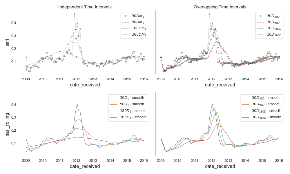
As mentioned before, by using the SHIFTperiod approach you can define both strategies to generate time-series (ITI and OTI). The ITI strategy is limited in the number of samples that can be used to compute the index and therefore you have to trade between granularity and accuracy whereas the latter is more flexible.
For instance, in examples with low number of records sari might
go up from barely 0.1 (in ITI) to 0.4 (in OTI) when more records are
used. The most noticeable increase from 1M1 to 1M3, that is when
instead of records for a month we considered records for three months
and reached certain stability on 1M6 approximately (ish?).
Note
Ideally shift and period same unit (eg. D).
Period should be always larger than shift.
278 # --------------------------------
279 # Comparison
280 # --------------------------------
281 # Configuration
282 shift = '30D'
283
284 # Create figure
285 f, axes = plt.subplots(2, 2, figsize=(10, 6), sharey=True)
286 axes = axes.flatten()
287
288 # Loop
289 for period in ['30D', '90D', '180D', '365D']:
290
291     # Compute sari time-series
292     iti = sar.compute(data, shift=period,
293         period=period, cdate='date_received')
294     oti = sar.compute(data, shift=shift,
295         period=period, cdate='date_received')
296
297     # Compute rolling mean
298     iti['sari_rolling'] = iti.sari.rolling(window=3,
299         win_type='gaussian', min_periods=1).mean(std=3)
300     oti['sari_rolling'] = oti.sari.rolling(window=3,
301         win_type='gaussian', min_periods=1).mean(std=3)
302
303     # Plot
304     sns.lineplot(data=iti, x='date_received', y='sari',
305                  linewidth=0.75, linestyle='--', ax=axes[0], marker='o',
306                  markersize=3, markeredgecolor='k', markeredgewidth=0.5,
307                  markerfacecolor=None, alpha=0.5,
308                  label='$%sM_{%s}$' % (period, 1))
309
310     sns.lineplot(data=oti, x='date_received', y='sari',
311                  linewidth=0.75, linestyle='--', ax=axes[1], marker='o',
312                  markersize=3, markeredgecolor='k', markeredgewidth=0.5,
313                  markerfacecolor=None, alpha=0.5,
314                  label='$%s_{%s}$' % (shift, period))
315
316     sns.lineplot(data=iti, x='date_received', y='sari_rolling',
317                  linewidth=0.75, ax=axes[2],
318                  label='$%s_{%s}$ - smooth' % (period, 1))
319
320     sns.lineplot(data=oti, x='date_received', y='sari_rolling',
321                  linewidth=0.75, ax=axes[3],
322                  label='$%s_{%s}$ - smooth' % (shift, period))
323
324 # Configure
325 sns.despine(bottom=True)
326
327 # Configure axes
328 axes[0].set(title='Independent Time Intervals')
329 axes[1].set(title='Overlapping Time Intervals')
330
331 # Adjust
332 plt.tight_layout()
333
334 # Show
335 plt.show()

Plotting multiple pairs using FaceGrid.
343 """
344 # ----------------------
345 # Facet Grid
346 # ----------------------
347 # Show
348 print(aux)
349
350 # Create palette
351 pal = sns.cubehelix_palette(50, rot=-.25, light=.7)
352
353 # Create
354 g = sns.FacetGrid(data=aux, col="antimicrobial_code",
355     hue="antimicrobial_code", aspect=1.2, height=2,
356     sharex=True, sharey=True, palette=pal,
357     col_wrap=8)
358
359 # Plot line
360 g.map(sns.lineplot, "date_received", 'sari',
361       alpha=1, linewidth=1.5)
362 """
363 """
364 g.map(plt.fill_between,
365       aux.date_received.values,
366       aux.sari.values)
367 """
368 """
369 #g.map(label, "x")
370 #g.set_titles("")
371 #g.set(yticks=[])
372 g.set(xlabel='date')
373 g.despine(bottom=True, left=True)
374
375 # Show
376 plt.show()
377 """
'\n#g.map(label, "x")\n#g.set_titles("")\n#g.set(yticks=[])\ng.set(xlabel=\'date\')\ng.despine(bottom=True, left=True)\n\n# Show\nplt.show()\n'
Total running time of the script: ( 0 minutes 15.742 seconds)