Step 01 - Compute AMR metrics

Loading susceptibility test data

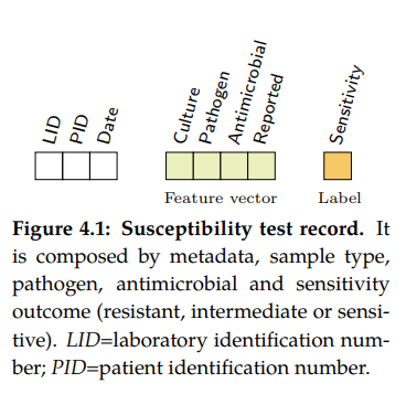
A Susceptibility test record (see figure 4.1) is composed by laboratory identification number (LID), patient identification number (PID), date, sample type, specimen or culture (e.g. blood or urine), pathogen, antimicrobial, reported status and outcome (resistant, sensitive or intermediate). In this research, the susceptibility test data were grouped firstly by specimen type. Moreover, for each sample type, the data were grouped by pairs (pathogen, antimicrobial) since it is widely accepted by clinicians as detailed in the UK five year strategy in AMR.

A small dataset will be used for this example.

# Libraries
import numpy as np
import pandas as pd
import seaborn as sns
import matplotlib as mpl
import matplotlib.pyplot as plt

# Import from pyAMR
from pyamr.datasets.load import make_susceptibility

try:
    __file__
    TERMINAL = True
except:
    TERMINAL = False

# -------------------------------------------
# Load data
# -------------------------------------------
# Load data
data = make_susceptibility()
data = data.drop_duplicates()

# Show
print("\nData:")
print(data)
print("\nColumns:")
print(data.dtypes)
print("\nUnique:")
print(data[[
    'microorganism_code',
    'antimicrobial_code',
    'specimen_code',
    'laboratory_number',
    'patient_id']].nunique())

Data:
       date_received  date_outcome  patient_id laboratory_number specimen_code  specimen_name specimen_description  ... microorganism_name antimicrobial_code antimicrobial_name sensitivity_method  sensitivity mic  reported
0         2009-01-03           NaN       20091           X428501        BLDCUL            NaN                blood  ...         klebsiella               AAMI           amikacin                NaN    sensitive NaN       NaN
1         2009-01-03           NaN       20091           X428501        BLDCUL            NaN                blood  ...         klebsiella               AAMO        amoxycillin                NaN    resistant NaN       NaN
2         2009-01-03           NaN       20091           X428501        BLDCUL            NaN                blood  ...         klebsiella               AAUG          augmentin                NaN    sensitive NaN       NaN
3         2009-01-03           NaN       20091           X428501        BLDCUL            NaN                blood  ...         klebsiella               AAZT          aztreonam                NaN    sensitive NaN       NaN
4         2009-01-03           NaN       20091           X428501        BLDCUL            NaN                blood  ...         klebsiella               ACAZ        ceftazidime                NaN    sensitive NaN       NaN
...              ...           ...         ...               ...           ...            ...                  ...  ...                ...                ...                ...                ...          ...  ..       ...
319117    2009-12-31           NaN       24645          H2012337        BLDCUL            NaN                blood  ...       enterococcus               AAMO        amoxycillin                NaN    sensitive NaN       NaN
319118    2009-12-31           NaN       24645          H2012337        BLDCUL            NaN                blood  ...       enterococcus               ALIN          linezolid                NaN    sensitive NaN       NaN
319119    2009-12-31           NaN       24645          H2012337        BLDCUL            NaN                blood  ...       enterococcus               ASYN           synercid                NaN    resistant NaN       NaN
319120    2009-12-31           NaN       24645          H2012337        BLDCUL            NaN                blood  ...       enterococcus               ATEI        teicoplanin                NaN    sensitive NaN       NaN
319121    2009-12-31           NaN       24645          H2012337        BLDCUL            NaN                blood  ...       enterococcus               AVAN         vancomycin                NaN    sensitive NaN       NaN

[319122 rows x 15 columns]

Columns:
date_received            object
date_outcome            float64
patient_id                int64
laboratory_number        object
specimen_code            object
specimen_name           float64
specimen_description     object
microorganism_code       object
microorganism_name       object
antimicrobial_code       object
antimicrobial_name       object
sensitivity_method      float64
sensitivity              object
mic                     float64
reported                float64
dtype: object

Unique:
microorganism_code       67
antimicrobial_code       58
specimen_code            22
laboratory_number     34816
patient_id            24646
dtype: int64

Computing SARI

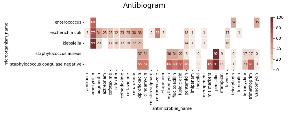
The Single Antimicrobial Resistance Index or SARI describes the proportion of resistant isolates for a given set of susceptibility tests. It provides a value within the range [0, 1] where values close to one indicate high resistance. It is agnostic to pathogen, antibiotic and/or time. The variables R, I and S represent the number of susceptibility tests with Resistant, Intermediate and Susceptible outcomes respectively. The definition might vary slightly since the intermediate category is not always considered.

For more information see: pyamr.core.sari.SARI

For more examples see:

• Single Antimicrobial Resistance (SARI)

• SARI - By specimen w/ sns.heatmap

• SARI - By specimen w/ sns.clustermap

• SARI - By specimen w/ sns.relmap

# -------------------------------------------
# Compute SARI
# -------------------------------------------
# Libraries
from pyamr.core.sari import SARI

# Create sari instance
sari = SARI(groupby=['specimen_code',
                     'microorganism_name',
                     'antimicrobial_name',
                     'sensitivity'])

# Compute SARI overall
sari_overall = sari.compute(data,
    return_frequencies=True)

# Show
print("SARI (overall):")
print(sari_overall)

# ------------
# Plot Heatmap
# ------------
# Filter
matrix = sari_overall.copy(deep=True)
matrix = matrix.reset_index()
matrix = matrix[matrix.freq > 100]
matrix = matrix[matrix.specimen_code.isin(['BLDCUL'])]

# Pivot table
matrix = pd.pivot_table(matrix,
    index='microorganism_name',
    columns='antimicrobial_name',
    values='sari')

# Create figure
f, ax = plt.subplots(1, 1, figsize=(10, 4))

# Create colormap
cmap = sns.color_palette("Reds", desat=0.5, n_colors=10)

# Plot
ax = sns.heatmap(data=matrix*100, annot=True, fmt=".0f",
    annot_kws={'fontsize': 'small'}, cmap=cmap,
    linewidth=0.5, vmin=0, vmax=100, ax=ax,
    xticklabels=1, yticklabels=1)

# Add title
plt.suptitle("Antibiogram", fontsize='xx-large')

# Tight layout
plt.tight_layout()
plt.subplots_adjust(right=1.05)

SARI (overall):
                                                                        intermediate  resistant  sensitive  freq      sari
specimen_code microorganism_name                    antimicrobial_name
BFLCUL        anaerobes                             metronidazole                0.0        0.0        1.0   1.0  0.000000
              bacillus                              ciprofloxacin                0.0        0.0        1.0   1.0  0.000000
                                                    clindamycin                  0.0        3.0        1.0   4.0  0.750000
                                                    erythromycin                 0.0        1.0        3.0   4.0  0.250000
                                                    fusidic acid                 0.0        3.0        1.0   4.0  0.750000
...                                                                              ...        ...        ...   ...       ...
XINCUL        streptococcus beta-haemolytic group b cephalexin                   0.0        1.0        0.0   1.0  1.000000
                                                    clindamycin                  0.0        1.0        8.0   9.0  0.111111
                                                    erythromycin                 0.0        1.0        8.0   9.0  0.111111
                                                    penicillin                   0.0        0.0        9.0   9.0  0.000000
                                                    tetracycline                 0.0        8.0        1.0   9.0  0.888889

[4491 rows x 5 columns]

Computing MARI

Warning

Pending… similar to SARI.

Computing ASAI

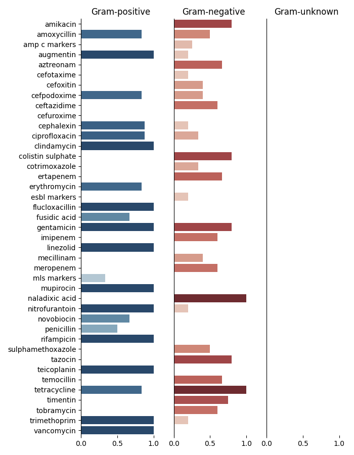
The antimicrobial spectrum of activity refers to the range of microbe species that are susceptible to these agents and therefore can be treated. In general, antimicrobial agents are classified into broad, intermediate or narrow spectrum. Broad spectrum antimicrobials are active against both Gram-positive and Gram-negative bacteria. In contrast, narrow spectrum antimicrobials have limited activity and are effective only against particular species of bacteria. While these profiles appeared in the mid-1950s, little effort has been made to define them. Furthermore, such ambiguous labels are overused for different and even contradictory purposes.

In order to compute the antimicrobial spectrum of activity index or ASAI, it is necessary to previously obtain the overall resistance (SARI) for all the microbe-antimicrobial pairs. Furthermore, by following the criteria used in the narrow-broad approach, these pairs were grouped into Gram-positive and Gram-negative. Briefly, the weighted proportion of species to which the antimicrobial is effective is computed for each genus. These are later added up and normalized by the number of genera tested. An antimicrobial is considered effective to treat a particular species when the corresponding resistance index (SARI) is lower than a given threshold.

For more information see: pyamr.core.asai.ASAI

For more examples see:

• ASAI - By gram stain (binary)

• ASAI - By gram stain (multiple)

In order to compute ASAI, we need to have the following columns present in our dataset: antimicrobial, microorganism_genus, microorganism_species and resistance. Moreover, in this example we will compute the ASAI for each gram_stain category independently so we will need the microorganism gram stain information too. This information is available in the registries: pyamr.datasets.registries

Lets include all this information using the MicroorganismRegistry.

# ------------------------------
# Include gram stain
# ------------------------------
# Libraries
from pyamr.datasets.registries import MicroorganismRegistry

# Load registry
mreg = MicroorganismRegistry()

# Format sari dataframe
dataframe = sari_overall.copy(deep=True)
dataframe = dataframe.reset_index()

# Create genus and species
dataframe[['genus', 'species']] = \
    dataframe.microorganism_name \
        .str.capitalize() \
        .str.split(expand=True, n=1)

# Combine with registry information
dataframe = mreg.combine(dataframe, on='microorganism_name')

# Fill missing gram stain
dataframe.gram_stain = dataframe.gram_stain.fillna('u')

Now that we have the genus, species and gram_stain information, lets compute ASAI.

# -------------------------------------------
# Compute ASAI
# -------------------------------------------
# Import specific libraries
from pyamr.core.asai import ASAI

# Create asai instance
asai = ASAI(column_genus='genus',
            column_specie='species',
            column_resistance='sari',
            column_frequency='freq')

# Compute
scores = asai.compute(dataframe,
    groupby=['specimen_code',
             'antimicrobial_name',
             'gram_stain'],
    weights='uniform',
    threshold=0.5,
    min_freq=0)

# Stack
scores = scores.unstack()

# Filter and drop index.
scores = scores.filter(like='URICUL', axis=0)
scores.index = scores.index.droplevel()

# Show
print("\nASAI (overall):")
print(scores)

c:\users\kelda\desktop\repositories\github\pyamr\main\pyamr\core\asai.py:572: UserWarning:


                 Extreme resistances [0, 1] were found in the DataFrame. These
                 rows should be reviewed since these resistances might correspond
                 to pairs with low number of records.


c:\users\kelda\desktop\repositories\github\pyamr\main\pyamr\core\asai.py:583: UserWarning:


                 There are NULL values in columns that are required. These
                 rows will be ignored to safely compute ASAI. Please review
                 the DataFrame and address this inconsistencies. See below
                 for more information:

                        specimen_code            0
                        antimicrobial_name       0
                        gram_stain               0
                        GENUS                    0
                        SPECIE                2414
                        RESISTANCE               0



ASAI (overall):
                   N_GENUS          N_SPECIE          ASAI_SCORE
gram_stain               n    p   u        n    p   u          n         p   u
antimicrobial_name
amikacin               5.0  NaN NaN      5.0  NaN NaN   0.800000       NaN NaN
amoxycillin            2.0  2.0 NaN      2.0  7.0 NaN   0.500000  0.833333 NaN
amp c markers          4.0  NaN NaN      4.0  NaN NaN   0.250000       NaN NaN
augmentin              5.0  2.0 NaN      5.0  7.0 NaN   0.200000  1.000000 NaN
aztreonam              3.0  NaN NaN      3.0  NaN NaN   0.666667       NaN NaN
cefotaxime             5.0  NaN NaN      5.0  NaN NaN   0.200000       NaN NaN
cefoxitin              5.0  NaN NaN      5.0  NaN NaN   0.400000       NaN NaN
cefpodoxime            5.0  2.0 NaN      5.0  5.0 NaN   0.400000  0.833333 NaN
ceftazidime            5.0  NaN NaN      5.0  NaN NaN   0.600000       NaN NaN
cefuroxime             5.0  NaN NaN      5.0  NaN NaN   0.000000       NaN NaN
cephalexin             5.0  2.0 NaN      5.0  7.0 NaN   0.200000  0.875000 NaN
ciprofloxacin          6.0  2.0 NaN      6.0  7.0 NaN   0.333333  0.875000 NaN
clindamycin            NaN  2.0 NaN      NaN  4.0 NaN        NaN  1.000000 NaN
colistin sulphate      5.0  NaN NaN      5.0  NaN NaN   0.800000       NaN NaN
cotrimoxazole          3.0  NaN NaN      3.0  NaN NaN   0.333333       NaN NaN
ertapenem              3.0  NaN NaN      3.0  NaN NaN   0.666667       NaN NaN
erythromycin           NaN  2.0 NaN      NaN  6.0 NaN        NaN  0.833333 NaN
esbl markers           5.0  NaN NaN      5.0  NaN NaN   0.200000       NaN NaN
flucloxacillin         1.0  1.0 NaN      1.0  3.0 NaN   0.000000  1.000000 NaN
fusidic acid           NaN  1.0 NaN      NaN  3.0 NaN        NaN  0.666667 NaN
gentamicin             5.0  1.0 NaN      5.0  3.0 NaN   0.800000  1.000000 NaN
imipenem               5.0  NaN NaN      5.0  NaN NaN   0.600000       NaN NaN
linezolid              NaN  1.0 NaN      NaN  3.0 NaN        NaN  1.000000 NaN
mecillinam             5.0  NaN NaN      5.0  NaN NaN   0.400000       NaN NaN
meropenem              5.0  NaN NaN      5.0  NaN NaN   0.600000       NaN NaN
mls markers            NaN  1.0 NaN      NaN  3.0 NaN        NaN  0.333333 NaN
mupirocin              NaN  1.0 NaN      NaN  2.0 NaN        NaN  1.000000 NaN
naladixic acid         1.0  NaN NaN      1.0  NaN NaN   1.000000       NaN NaN
nitrofurantoin         5.0  2.0 NaN      5.0  7.0 NaN   0.200000  1.000000 NaN
novobiocin             1.0  1.0 NaN      1.0  3.0 NaN   0.000000  0.666667 NaN
penicillin             1.0  2.0 NaN      1.0  6.0 NaN   0.000000  0.500000 NaN
rifampicin             NaN  1.0 NaN      NaN  3.0 NaN        NaN  1.000000 NaN
sulphamethoxazole      2.0  NaN NaN      2.0  NaN NaN   0.500000       NaN NaN
tazocin                5.0  NaN NaN      5.0  NaN NaN   0.800000       NaN NaN
teicoplanin            NaN  2.0 NaN      NaN  7.0 NaN        NaN  1.000000 NaN
temocillin             3.0  NaN NaN      3.0  NaN NaN   0.666667       NaN NaN
tetracycline           1.0  2.0 NaN      1.0  6.0 NaN   1.000000  0.833333 NaN
timentin               4.0  NaN NaN      4.0  NaN NaN   0.750000       NaN NaN
tobramycin             5.0  NaN NaN      5.0  NaN NaN   0.600000       NaN NaN
trimethoprim           5.0  2.0 NaN      5.0  7.0 NaN   0.200000  1.000000 NaN
vancomycin             NaN  2.0 NaN      NaN  7.0 NaN        NaN  1.000000 NaN

This is the information obtained where the columns n, p, and u stand for gram-positive, gram-negative and unknown respectively. Similarly, N_GENUS and N_SPECIE indicates the number of genus and species for the specific antimicrobial.

scores.head(10)

	N_GENUS			N_SPECIE			ASAI_SCORE
gram_stain	n	p	u	n	p	u	n	p	u
antimicrobial_name
amikacin	5.0	NaN	NaN	5.0	NaN	NaN	0.800000	NaN	NaN
amoxycillin	2.0	2.0	NaN	2.0	7.0	NaN	0.500000	0.833333	NaN
amp c markers	4.0	NaN	NaN	4.0	NaN	NaN	0.250000	NaN	NaN
augmentin	5.0	2.0	NaN	5.0	7.0	NaN	0.200000	1.000000	NaN
aztreonam	3.0	NaN	NaN	3.0	NaN	NaN	0.666667	NaN	NaN
cefotaxime	5.0	NaN	NaN	5.0	NaN	NaN	0.200000	NaN	NaN
cefoxitin	5.0	NaN	NaN	5.0	NaN	NaN	0.400000	NaN	NaN
cefpodoxime	5.0	2.0	NaN	5.0	5.0	NaN	0.400000	0.833333	NaN
ceftazidime	5.0	NaN	NaN	5.0	NaN	NaN	0.600000	NaN	NaN
cefuroxime	5.0	NaN	NaN	5.0	NaN	NaN	0.000000	NaN	NaN

Lets plot it now!

# ---------------------------------------------------------------
# Plot
# ---------------------------------------------------------------
# .. note: In order to sort the scores we need to compute metrics
#          that combine the different subcategories (e.g. gram-negative
#          and gram-positive). Two possible options are: (i) use the
#          gmean or (ii) the width.

# Libraries
from pyamr.utils.plot import scalar_colormap

# Measures
scores['width'] = np.abs(scores['ASAI_SCORE'].sum(axis=1))

# Variables to plot.
x = scores.index.values
y_n = scores['ASAI_SCORE']['n'].values
y_p = scores['ASAI_SCORE']['p'].values
y_u = scores['ASAI_SCORE']['u'].values

# Constants
colormap_p = scalar_colormap(y_p, cmap='Blues', vmin=-0.1, vmax=1.1)
colormap_n = scalar_colormap(y_n, cmap='Reds', vmin=-0.1, vmax=1.1)
colormap_u = scalar_colormap(y_u, cmap='Greens', vmin=-0.1, vmax=1.1)

# ----------
# Example
# ----------
# This example shows an stacked figure using more than two categories.
# For instance, it uses gram-positive, gram-negative and gram-unknown.
# All the indexes go within the range [0,1].
# Create the figure
f, axes = plt.subplots(1, 3, figsize=(7, 9))

# Plot each category
sns.barplot(x=y_p, y=x, palette=colormap_p, ax=axes[0], orient='h',
            saturation=0.5, label='Gram-positive')
sns.barplot(x=y_n, y=x, palette=colormap_n, ax=axes[1], orient='h',
            saturation=0.5, label='Gram-negative')
sns.barplot(x=y_u, y=x, palette=colormap_u, ax=axes[2], orient='h',
            saturation=0.5, label='Gram-unknown')

# Configure
sns.despine(bottom=True)

# Format figure
plt.subplots_adjust(wspace=0.0, hspace=0.0)

# Remove yticks
axes[1].set_yticks([])
axes[2].set_yticks([])

# Set title
axes[0].set_title('Gram-positive')
axes[1].set_title('Gram-negative')
axes[2].set_title('Gram-unknown')

# Set x-axis
axes[0].set_xlim([0, 1.1])
axes[1].set_xlim([0, 1.1])
axes[2].set_xlim([0, 1.1])

# Adjust
plt.tight_layout()

Computing SART

The single antimicrobial resistance trend or SART measures the ratio of change per time unit (e.g. monthly or yearly). To compute this metric, it is necessary to generate a resistance time series from the susceptibility test data. This is often achieved by computing the SARI on consecutive or overlapping partitions of the data. Then, the trend can be extracted using for example a linear model where the slope, which is represented by a value within the range [-1, 1], indicates the ratio of change.

For more information see: pyamr.core.sart.SART

For more examples see:

• Single Resistance Trend (SART)

• SART - Trend as slope of WLS

Note

Be cautious when computing the SART index using a small dataset (e.g. a low number of susceptibility tests records) since it is very likely that the statistics produced (e.g. kurtosis or skewness) will be ill defined. Also remember to check stationarity if using ARIMA.

Since it is necessary to have a decent amount of records to be able to compute the trends accurately, lets see which tuples have more number of samples.

# -------------------------------------------
# Show top combinations
# -------------------------------------------
from pyamr.core.sari import SARI

# Create SARI instance
sar = SARI(groupby=['specimen_code',
                    'microorganism_code',
                    'antimicrobial_code',
                    'sensitivity'])

# Compute SARI overall
sari_overall = sar.compute(data,
     return_frequencies=True)

# Compute top tuples
top = sari_overall \
    .sort_values(by='freq', ascending=False) \
    .head(10)

# Show
print("\nTop by Frequency:")
print(top)

Top by Frequency:
                                                     intermediate  resistant  sensitive    freq      sari
specimen_code microorganism_code antimicrobial_code
URICUL        ECOL               A_CEFPODOX                   0.0      595.0     8582.0  9177.0  0.064836
                                 ANIT                         0.0      347.0     8826.0  9173.0  0.037828
                                 ACELX                        0.0      803.0     8370.0  9173.0  0.087540
                                 ATRI                         0.0     3231.0     5941.0  9172.0  0.352268
                                 ACIP                         0.0     1259.0     7913.0  9172.0  0.137266
                                 AAUG                         0.0      602.0     8561.0  9163.0  0.065699
WOUCUL        SAUR               AFUS                         0.0      613.0     3631.0  4244.0  0.144439
                                 APEN                         0.0     3677.0      566.0  4243.0  0.866604
                                 AERY                         0.0     1186.0     3056.0  4242.0  0.279585
                                 AMET                         0.0      869.0     3372.0  4241.0  0.204905

Let’s choose the tuples were are interested in.

# -------------------------------------------
# Filter data
# -------------------------------------------
# Define spec, orgs, abxs of interest
spec = ['URICUL']
orgs = ['ECOL']
abxs = ['ACELX', 'ACIP', 'AAMPC', 'ATRI', 'AAUG',
        'AMER', 'ANIT', 'AAMI', 'ACTX', 'ATAZ',
        'AGEN', 'AERT', 'ACAZ', 'AMEC', 'ACXT']

# Create auxiliary DataFrame
aux = data.copy(deep=True) \

# Filter
idxs_spec = data.specimen_code.isin(spec)
idxs_orgs = data.microorganism_code.isin(orgs)
idxs_abxs = data.antimicrobial_code.isin(abxs)

# Filter
aux = aux[idxs_spec & idxs_orgs & idxs_abxs]

Now, lets compute the resistance trend.

# Libraries
import warnings

# Import specific libraries
from pyamr.core.sart import SART

# Variables
shift, period = '10D', '180D'

# Create instance
sar = SART(column_specimen='specimen_code',
           column_microorganism='microorganism_code',
           column_antimicrobial='antimicrobial_code',
           column_date='date_received',
           column_outcome='sensitivity',
           column_resistance='sari')

with warnings.catch_warnings():
    warnings.simplefilter('ignore')

    # Compute resistance trends
    table, objs = sar.compute(aux, shift=shift,
        period=period, return_objects=True)

 1/15. Computing... ('URICUL', 'ECOL', 'AAMI')
 2/15. Computing... ('URICUL', 'ECOL', 'AAMPC')
 3/15. Computing... ('URICUL', 'ECOL', 'AAUG')
 4/15. Computing... ('URICUL', 'ECOL', 'ACAZ')
 5/15. Computing... ('URICUL', 'ECOL', 'ACELX')
 6/15. Computing... ('URICUL', 'ECOL', 'ACIP')
 7/15. Computing... ('URICUL', 'ECOL', 'ACTX')
 8/15. Computing... ('URICUL', 'ECOL', 'ACXT')
 9/15. Computing... ('URICUL', 'ECOL', 'AERT')
10/15. Computing... ('URICUL', 'ECOL', 'AGEN')
11/15. Computing... ('URICUL', 'ECOL', 'AMEC')
12/15. Computing... ('URICUL', 'ECOL', 'AMER')
13/15. Computing... ('URICUL', 'ECOL', 'ANIT')
14/15. Computing... ('URICUL', 'ECOL', 'ATAZ')
15/15. Computing... ('URICUL', 'ECOL', 'ATRI')

Lets see the results(note it is transposed!)

# Configure pandas
pd.set_option(
    'display.max_colwidth', 20,
    'display.width', 1000
)

# Show
#print("Results:")
#print(table.T)
table.head(4).T

specimen_code	URICUL
microorganism_code	ECOL
antimicrobial_code	AAMI	AAMPC	AAUG	ACAZ
wls-rsquared	0.557029	0.12798	0.906452	0.004545
wls-rsquared_adj	0.544373	0.09791	0.903779	-0.023896
wls-fvalue	44.012024	4.256121	339.140633	0.159818
wls-fprob	0.0	0.048164	0.0	0.691754
wls-aic	inf	inf	inf	inf
wls-bic	inf	inf	inf	inf
wls-llf	-inf	-inf	-inf	-inf
wls-mse_model	0.745856	4.978205	33.299393	0.2007
wls-mse_resid	0.016947	1.169658	0.098188	1.255805
wls-mse_total	0.037194	1.296609	1.020443	1.226496
wls-const_coef	0.031283	68.761679	1.544961	65.712841
wls-const_std	0.093007	0.698295	0.234858	0.80353
wls-const_tvalue	0.336351	98.470788	6.578289	81.780194
wls-const_tprob	0.738614	0.0	0.0	0.0
wls-const_cil	-0.157532	67.333505	1.068175	64.081588
wls-const_ciu	0.220098	70.189854	2.021747	67.344094
wls-x1_coef	0.024239	0.072052	0.167941	-0.012606
wls-x1_std	0.003654	0.034925	0.009119	0.031532
wls-x1_tvalue	6.634156	2.063037	18.415771	-0.399772
wls-x1_tprob	0.0	0.048164	0.0	0.691754
wls-x1_cil	0.016822	0.000622	0.149427	-0.076619
wls-x1_ciu	0.031656	0.143482	0.186454	0.051408
wls-s_dw	0.741	1.091	0.176	0.445
wls-s_jb_value	0.509	0.638	2.336	0.239
wls-s_jb_prob	0.775	0.727	0.311	0.887
wls-s_skew	0.21	-0.17	0.316	-0.051
wls-s_kurtosis	2.608	2.385	1.944	2.62
wls-s_omnibus_value	0.39	0.518	5.037	0.05
wls-s_omnibus_prob	0.823	0.772	0.081	0.975
wls-m_dw	0.736178	0.537678	0.043909	0.188735
wls-m_jb_value	26.465944	457.685847	27.729537	10.593247
wls-m_jb_prob	0.000002	0.0	0.000001	0.005008
wls-m_skew	1.61218	4.04353	1.89606	1.267125
wls-m_kurtosis	5.602039	19.998144	4.899094	3.66998
wls-m_nm_value	19.984589	59.422218	21.39435	10.974889
wls-m_nm_prob	0.000046	0.0	0.000023	0.004138
wls-m_ks_value	0.405236	0.149246	0.366502	0.365003
wls-m_ks_prob	0.000005	0.451309	0.000058	0.000063
wls-m_shp_value	0.845794	0.486878	0.565564	0.844264
wls-m_shp_prob	0.000126	0.0	0.0	0.000116
wls-m_ad_value	1.637801	5.197208	7.445695	2.187059
wls-m_ad_nnorm	False	False	False	False
wls-pearson	0.548657	-0.482852	-0.197034	-0.816642
wls-missing	raise	raise	raise	raise
wls-exog	[[1.0, 0.0], [1....	[[1.0, 0.0], [1....	[[1.0, 0.0], [1....	[[1.0, 0.0], [1....
wls-endog	[0.0, 0.0, 0.0, ...	[100.0, 77.77777...	[13.513513513513...	[75.0, 73.529411...
wls-trend	c	c	c	c
wls-weights	[0.0, 0.00281585...	[0.0, 0.03706907...	[0.0, 0.00124501...	[0.0, 0.00278805...
wls-W	<pyamr.metrics.w...	<pyamr.metrics.w...	<pyamr.metrics.w...	<pyamr.metrics.w...
wls-model	<statsmodels.reg...	<statsmodels.reg...	<statsmodels.reg...	<statsmodels.reg...
wls-id	WLS(c,Sig(N, N))	WLS(c,Sig(N, N))	WLS(c,Sig(N, N))	WLS(c,Sig(N, N))

Lets visualise the first entry

# Display
# This example shows how to make predictions using the wrapper and how
# to plot the result in data. In addition, it compares the intervals
# provided by get_prediction (confidence intervals) and the intervals
# provided by wls_prediction_std (prediction intervals).

# Variables
name, obj = objs[2] # AAUG

# Series
series = obj.as_series()

# Variables.
start, end = None, 50

# Get x and y
x = series['wls-exog'][:,1]
y = series['wls-endog']

# Compute predictions (exogenous?). It returns a 2D array
# where the rows contain the time (t), the mean, the lower
# and upper confidence (or prediction?) interval.
preds = obj.get_prediction(start=start, end=end)

# Create figure
fig, ax = plt.subplots(1, 1, figsize=(11, 5))

# Plotting confidence intervals
# -----------------------------
# Plot truth values.
ax.plot(x, y, color='#A6CEE3', alpha=0.5, marker='o',
        markeredgecolor='k', markeredgewidth=0.5,
        markersize=5, linewidth=0.75, label='Observed')

# Plot forecasted values.
ax.plot(preds[0, :], preds[1, :], color='#FF0000', alpha=1.00,
        linewidth=2.0, label=obj._identifier(short=True))

# Plot the confidence intervals.
ax.fill_between(preds[0, :], preds[2, :],
                preds[3, :],
                color='r',
                alpha=0.1)

# Legend
plt.legend()
plt.title(name)

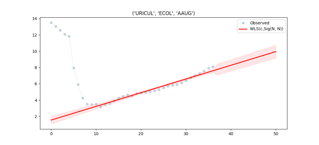
Text(0.5, 1.0, "('URICUL', 'ECOL', 'AAUG')")

Lets see the summary

# Summary
print("Name: %s\n" % str(name))
print(obj.as_summary())

Name: ('URICUL', 'ECOL', 'AAUG')

                            WLS Regression Results
==============================================================================
Dep. Variable:                      y   R-squared:                       0.906
Model:                            WLS   Adj. R-squared:                  0.904
Method:                 Least Squares   F-statistic:                     339.1
Date:                Thu, 15 Jun 2023   Prob (F-statistic):           1.38e-19
Time:                        18:15:41   Log-Likelihood:                   -inf
No. Observations:                  37   AIC:                               inf
Df Residuals:                      35   BIC:                               inf
Df Model:                           1
Covariance Type:            nonrobust
==============================================================================
                 coef    std err          t      P>|t|      [0.025      0.975]
------------------------------------------------------------------------------
const          1.5450      0.235      6.578      0.000       1.068       2.022
x1             0.1679      0.009     18.416      0.000       0.149       0.186
==============================================================================
Omnibus:                        5.037   Durbin-Watson:                   0.176
Prob(Omnibus):                  0.081   Jarque-Bera (JB):                2.336
Skew:                           0.316   Prob(JB):                        0.311
Kurtosis:                       1.944   Cond. No.                         91.7
Normal (N):                    21.394   Prob(N):                         0.000
==============================================================================

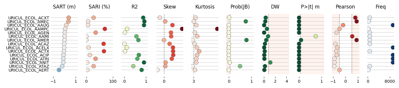
Lets display the information as a table graph for all tuples

# Libraries
from pyamr.graphics.table_graph import _DEFAULT_CONFIGURATION
from pyamr.graphics.table_graph import vlinebgplot

# Configuration for display
info = _DEFAULT_CONFIGURATION

# Lets define one as an example.
info['freq'] = {
    'cmap': 'Blues',
    'title': 'Freq',
    'xticks': [0, 8000],
    'kwargs': {
        's': 80,
        'vmin': 0
    }
}

# .. note: It is important to ensure that the column names
#          match with the keys of the previously loaded
#          info configuration so that it is used.

# Rename columns
rename = {
    'wls-x1_coef': 'sart_m',
    'wls-const_coef': 'offset',
    'wls-rsquared': 'r2',
    'wls-rsquared_adj': 'r2_adj',
    'wls-m_skew': 'skew',
    'wls-m_kurtosis': 'kurtosis',
    'wls-m_jb_prob': 'jb',
    'wls-m_dw': 'dw',
    'wls-const_tprob': 'ptm',
    'wls-x1_tprob': 'ptn',
    'wls-pearson': 'pearson',
    'freq': 'freq',
}


# ----------------
# Combine with SARI

# Format combined DataFrame
comb = table.join(sari_overall)
comb.index = comb.index.map('_'.join)
comb = comb.reset_index()
comb = comb.rename(columns=rename)

# Add new columns
comb['sart_y'] = comb.sart_m * 12   # Yearly trend
comb['sari_pct'] = comb.sari * 100  # SARI percent

# Sort by trend
comb = comb.sort_values(by='sart_y', ascending=False)

# Select only numeric columns
# data = comb.select_dtypes(include=np.number)
data = comb[[
    'index',
    'sart_m',
    #'sart_y',
    'sari_pct',
    'r2',
    #'r2_adj',
    'skew',
    'kurtosis',
    'jb',
    'dw',
    'ptm',
    #'ptn',
    'pearson',
    'freq'
]]

# Show DataFrame
#print("\nResults:")
#print(data)

# Create pair grid
g = sns.PairGrid(data, x_vars=data.columns[1:],
    y_vars=["index"], height=3, aspect=.45)

# Set common features
g.set(xlabel='', ylabel='')

# Plot strips and format axes (skipping index)
for ax, c in zip(g.axes.flat, data.columns[1:]):

    # Get information
    d = info[c] if c in info else {}

    # .. note: We need to use scatter plot if we want to
    #          assign colors to the markers according to
    #          their value.

    # Using scatter plot
    sns.scatterplot(data=data, x=c, y='index', s=100,
                    ax=ax, linewidth=0.75, edgecolor='gray',
                    c=data[c], cmap=d.get('cmap', None),
                    norm=d.get('norm', None))

    # Plot vertical lines
    for e in d.get('vline', []):
        vlinebgplot(ax, top=data.shape[0], **e)

    # Configure axes
    ax.set(title=d.get('title', c),
           xlim=d.get('xlim', None),
           xticks=d.get('xticks', []),
           xlabel='', ylabel='')
    ax.tick_params(axis='y', which='both', length=0)
    ax.xaxis.grid(False)
    ax.yaxis.grid(visible=True, which='major',
                  color='gray', linestyle='-', linewidth=0.35)

# Despine
sns.despine(left=True, bottom=True)

# Adjust layout
plt.tight_layout()
plt.show()

#%
# Lets see the data plotted
data.round(decimals=3)

	index	sart_m	sari_pct	r2	skew	kurtosis	jb	dw	ptm	pearson	freq
7	URICUL_ECOL_ACXT	0.385	27.961	0.872	-0.902	4.451	0.016	0.322	0.000	0.801	726.0
10	URICUL_ECOL_AMEC	0.364	6.923	0.925	0.292	3.163	0.753	0.247	0.000	0.905	390.0
2	URICUL_ECOL_AAUG	0.168	6.570	0.906	1.896	4.899	0.000	0.044	0.000	-0.197	9163.0
1	URICUL_ECOL_AAMPC	0.072	70.079	0.128	4.044	19.998	0.000	0.538	0.000	-0.483	254.0
9	URICUL_ECOL_AGEN	0.042	35.586	0.028	1.569	4.015	0.000	0.042	0.000	-0.726	725.0
0	URICUL_ECOL_AAMI	0.024	0.693	0.557	1.612	5.602	0.000	0.736	0.739	0.549	722.0
11	URICUL_ECOL_AMER	0.020	0.414	0.648	0.021	2.439	0.784	0.411	0.089	0.902	724.0
3	URICUL_ECOL_ACAZ	-0.013	65.522	0.005	1.267	3.670	0.005	0.189	0.000	-0.817	728.0
4	URICUL_ECOL_ACELX	-0.015	8.754	0.112	2.012	5.358	0.000	0.052	0.000	-0.664	9173.0
6	URICUL_ECOL_ACTX	-0.032	66.803	0.030	2.046	7.029	0.000	0.145	0.000	-0.746	732.0
5	URICUL_ECOL_ACIP	-0.075	13.727	0.669	2.075	5.565	0.000	0.071	0.000	-0.710	9172.0
14	URICUL_ECOL_ATRI	-0.093	35.227	0.600	1.751	4.933	0.000	0.089	0.000	-0.893	9172.0
12	URICUL_ECOL_ANIT	-0.094	3.783	0.907	0.369	4.881	0.043	1.134	0.000	-0.893	9173.0
13	URICUL_ECOL_ATAZ	-0.190	27.885	0.413	0.307	2.277	0.500	0.186	0.000	-0.911	728.0
8	URICUL_ECOL_AERT	-0.472	4.569	0.798	-1.436	3.976	0.001	0.078	0.000	-0.483	197.0

Computing ACSI

Warning

Pending…

Computing DRI

Warning

Pending…