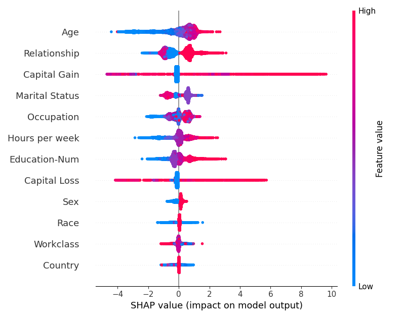
07. SHAP Beeswarm Plot

This script provides a concise, fundamental example of how to generate a SHAP beeswarm plot to visualize global feature importance. 🤖 It trains an XGBoost classifier on the adult census dataset, computes SHAP values, and then creates the classic beeswarm summary plot, which displays the impact of the most influential features on the model’s output.

Out:

 16%|===                 | 5193/32561 [00:11<00:57]
 18%|====                | 5710/32561 [00:12<00:56]
 19%|====                | 6227/32561 [00:13<00:54]
 21%|====                | 6741/32561 [00:14<00:53]
 22%|====                | 7240/32561 [00:15<00:52]
 24%|=====               | 7668/32561 [00:16<00:51]
 25%|=====               | 8146/32561 [00:17<00:50]
 27%|=====               | 8631/32561 [00:18<00:49]
 28%|======              | 9094/32561 [00:19<00:49]
 29%|======              | 9560/32561 [00:20<00:48]
 31%|======              | 10016/32561 [00:21<00:47]
 32%|======              | 10500/32561 [00:22<00:46]
 34%|=======             | 11012/32561 [00:23<00:45]
 35%|=======             | 11445/32561 [00:24<00:44]
 37%|=======             | 11885/32561 [00:25<00:43]
 38%|========            | 12378/32561 [00:26<00:42]
 39%|========            | 12829/32561 [00:27<00:41]
 41%|========            | 13284/32561 [00:28<00:40]
 42%|========            | 13710/32561 [00:29<00:39]
 44%|=========           | 14168/32561 [00:30<00:38]
 45%|=========           | 14660/32561 [00:31<00:37]
 47%|=========           | 15169/32561 [00:32<00:36]
 48%|==========          | 15645/32561 [00:33<00:35]
 49%|==========          | 16021/32561 [00:34<00:35]
 50%|==========          | 16419/32561 [00:35<00:34]
 52%|==========          | 16847/32561 [00:36<00:33]
 53%|===========         | 17317/32561 [00:37<00:32]
 55%|===========         | 17819/32561 [00:38<00:31]
 56%|===========         | 18325/32561 [00:39<00:30]
 58%|============        | 18750/32561 [00:40<00:29]
 59%|============        | 19181/32561 [00:41<00:28]
 60%|============        | 19601/32561 [00:42<00:27]
 62%|============        | 20065/32561 [00:43<00:26]
 63%|=============       | 20545/32561 [00:44<00:25]
 65%|=============       | 21027/32561 [00:45<00:24]
 66%|=============       | 21512/32561 [00:46<00:23]
 68%|==============      | 22008/32561 [00:47<00:22]
 69%|==============      | 22438/32561 [00:48<00:21]
 70%|==============      | 22880/32561 [00:49<00:20]
 72%|==============      | 23321/32561 [00:50<00:19]
 73%|===============     | 23813/32561 [00:51<00:18]
 75%|===============     | 24315/32561 [00:52<00:17]
 76%|===============     | 24832/32561 [00:53<00:16]
 78%|================    | 25348/32561 [00:54<00:15]
 79%|================    | 25857/32561 [00:55<00:14]
 81%|================    | 26375/32561 [00:56<00:13]
 83%|=================   | 26891/32561 [00:57<00:12]
 84%|=================   | 27403/32561 [00:58<00:10]
 86%|=================   | 27917/32561 [00:59<00:09]
 87%|=================   | 28433/32561 [01:00<00:08]
 89%|==================  | 28946/32561 [01:01<00:07]
 90%|==================  | 29463/32561 [01:02<00:06]
 92%|==================  | 29978/32561 [01:03<00:05]
 94%|=================== | 30485/32561 [01:04<00:04]
 95%|=================== | 30981/32561 [01:05<00:03]
 96%|=================== | 31381/32561 [01:06<00:02]
 98%|===================| 31854/32561 [01:07<00:01]
 99%|===================| 32367/32561 [01:08<00:00]       C:\Users\kelda\Desktop\repositories\virtualenvs\venv-py311-psc\Lib\site-packages\shap\plots\_beeswarm.py:503: UserWarning:

FigureCanvasAgg is non-interactive, and thus cannot be shown

# Libraries
import xgboost
import shap
import matplotlib.pyplot as plt

# Load shap dataset
X, y = shap.datasets.adult()

# Train model
model = xgboost.XGBClassifier().fit(X, y)

# Create shap explainer
explainer = shap.Explainer(model, X)
shap_values = explainer(X)

# Create beeswarm plot using explainer
shap.plots.beeswarm(shap_values,
    max_display=12,
    order=shap.Explanation.abs.mean(0))

# Adjust
plt.tight_layout()