Note
Click here to download the full example code
05. Display SHAP for Sequential Data
This script provides an in-depth guide on visualizing SHAP values for sequential or time-series data, a common challenge when interpreting models like LSTMs or other RNNs. It explores various techniques to break down and display the complex, three-dimensional SHAP output (samples, timesteps, features).
The script demonstrates several approaches:
Slicing SHAP Data: It shows how to use the standard
shap.summary_plotby systematically slicing the data, visualizing feature importances either per-timestep or across all timesteps for a single feature.Custom Seaborn Plots: It implements custom visualizations using
seaborn.stripplotandseaborn.swarmplotto offer more granular control over the plot’s appearance and layout.Advanced Coloring: Helper functions are created to replicate SHAP’s signature feature—coloring data points by their original feature value—allowing for richer interpretation in custom plots.
This example is a valuable resource for anyone looking to move beyond default plots and create tailored, insightful SHAP visualizations for models that handle sequential data.
 30 # Libraries
 31 import shap
 32 import numpy as np
 33 import pandas as pd
 34 import seaborn as sns
 35
 36 import matplotlib.pyplot as plt
 37 import matplotlib as mpl
 38 import matplotlib.colorbar
 39 import matplotlib.colors
 40 import matplotlib.cm
 41
 42 from mpl_toolkits.axes_grid1 import make_axes_locatable
 43
 44 try:
 45     __file__
 46     TERMINAL = True
 47 except:
 48     TERMINAL = False
 49
 50 # ------------------------
 51 # Methods
 52 # ------------------------
 53 def scalar_colormap(values, cmap, vmin, vmax):
 54     """This method creates a colormap based on values.
 55
 56     Parameters
 57     ----------
 58     values : array-like
 59     The values to create the corresponding colors
 60
 61     cmap : str
 62     The colormap
 63
 64     vmin, vmax : float
 65     The minimum and maximum possible values
 66
 67     Returns
 68     -------
 69     scalar colormap
 70     """
 71     # Create scalar mappable
 72     norm = mpl.colors.Normalize(vmin=vmin, vmax=vmax, clip=True)
 73     mapper = mpl.cm.ScalarMappable(norm=norm, cmap=cmap)
 74     # Get color map
 75     colormap = sns.color_palette([mapper.to_rgba(i) for i in values])
 76     # Return
 77     return colormap, norm
 78
 79
 80 def scalar_palette(values, cmap, vmin, vmax):
 81     """This method creates a colorpalette based on values.
 82
 83     Parameters
 84     ----------
 85     values : array-like
 86     The values to create the corresponding colors
 87
 88     cmap : str
 89     The colormap
 90
 91     vmin, vmax : float
 92     The minimum and maximum possible values
 93
 94     Returns
 95     -------
 96     scalar colormap
 97
 98     """
 99     # Create a matplotlib colormap from name
100     #cmap = sns.light_palette(cmap, reverse=False, as_cmap=True)
101     cmap = sns.color_palette(cmap, as_cmap=True)
102     # Normalize to the range of possible values from df["c"]
103     norm = mpl.colors.Normalize(vmin=vmin, vmax=vmax)
104     # Create a color dictionary (value in c : color from colormap)
105     colors = {}
106     for cval in values:
107         colors.update({cval : cmap(norm(cval))})
108     # Return
109     return colors, norm
110
111
112 def create_random_shap(samples, timesteps, features):
113     """Create random LSTM data.
114
115     .. note: No need to create the 3D matrix and then reshape to
116              2D. It would be possible to create directly the 2D
117              matrix.
118
119     Parameters
120     ----------
121     samples: int
122         The number of observations
123     timesteps: int
124         The number of time steps
125     features: int
126         The number of features
127
128     Returns
129     -------
130     Stacked matrix with the data.
131
132     """
133     # .. note: Either perform a pre-processing step such as
134     #          normalization or generate the features within
135     #          the appropriate interval.
136     # Create dataset
137     x = np.random.randint(low=0, high=100,
138         size=(samples, timesteps, features))
139     y = np.random.randint(low=0, high=2, size=samples).astype(float)
140     i = np.vstack(np.dstack(np.indices((samples, timesteps))))
141
142     # Create DataFrame
143     df = pd.DataFrame(
144         data=np.hstack((i, x.reshape((-1, features)))),
145         columns=['sample', 'timestep'] + \
146                 ['f%s'%j for j in range(features)]
147     )
148
149     df_stack = df.set_index(['sample', 'timestep']).stack()
150     df_stack = df_stack
151     df_stack.name = 'shap_values'
152     df_stack = df_stack.to_frame()
153     df_stack.index.names = ['sample', 'timestep', 'features']
154     df_stack = df_stack.reset_index()
155
156     df_stack['feature_values'] = np.random.randint(
157         low=0, high=100, size=df_stack.shape[0])
158
159     return df_stack
160
161
162 def load_shap_file():
163     data = pd.read_csv('./data/shap.csv')
164     data = data.iloc[: , 1:]
165     #data.timestep = data.timestep - (data.timestep.nunique() - 1)
166     return data
Lets generate and/or load the shap values.
171 # .. note: The right format to use for plotting depends
172 #          on the library we use. The data structure is
173 #          good when using seaborn
174 # Load data
175 data = create_random_shap(10, 6, 4)
176 #data = load_shap_file()
177 #data = data[data['sample'] < 100]
178
179 shap_values = pd.pivot_table(data,
180         values='shap_values',
181         index=['sample', 'timestep'],
182         columns=['features'])
183
184 feature_values = pd.pivot_table(data,
185         values='feature_values',
186         index=['sample', 'timestep'],
187         columns=['features'])
188
189 # Show
190 if TERMINAL:
191     print("\nShow:")
192     print(data)
193     print(shap_values)
194     print(feature_values)
Let’s see how data looks like
198 data.head(10)
Let’s see how shap_values looks like
202 shap_values.iloc[:10, :5]
Let’s see how feature_values looks like
206 feature_values.iloc[:10, :5]
Display using shap.summary_plot
The first option is to use the shap library to plot the results.
215 # Let's define/extract some useful variables.
216 N = 4                                                       # max loops filter
217 TIMESTEPS = len(shap_values.index.unique(level='timestep')) # number of timesteps
218 SAMPLES = len(shap_values.index.unique(level='sample'))     # number of samples
219
220 shap_min = data.shap_values.min()
221 shap_max = data.shap_values.max()
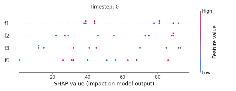
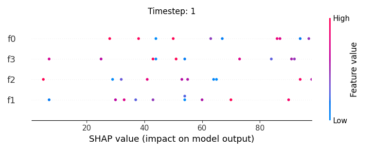
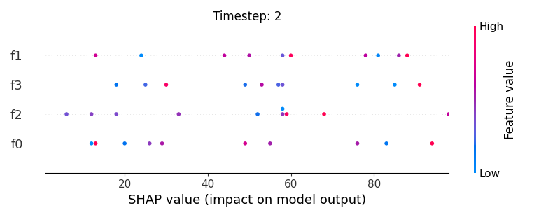
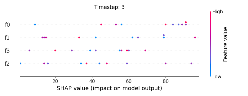
Now, let’s display the shap values for all features in each timestep.
226 # For each timestep (visualise all features)
227 for i, step in enumerate(range(TIMESTEPS)[:N]):
228     # Show
229     #print('%2d. %s' % (i, step))
230
231     # .. note: First option (commented) is only necessary if we work
232     #          with a numpy array. However, since we are using a DataFrame
233     #          with the timestep, we can index by that index level.
234     # Compute indices
235     #indice = np.arange(SAMPLES)*TIMESTEPS + step
236     indice = shap_values.index.get_level_values('timestep') == i
237
238     # Create auxiliary matrices
239     shap_aux = shap_values.iloc[indice]
240     feat_aux = feature_values.iloc[indice]
241
242     # Display
243     plt.figure()
244     plt.title("Timestep: %s" % i)
245     shap.summary_plot(shap_aux.to_numpy(), feat_aux, show=False)
246     plt.xlim(shap_min, shap_max)
Now, let’s display the shap values for all timesteps of each feature.
251 # For each feature (visualise all time-steps)
252 for i, f in enumerate(shap_values.columns[:N]):
253     # Show
254     #print('%2d. %s' % (i, f))
255
256     # Create auxiliary matrices (select feature and reshape)
257     shap_aux = shap_values.iloc[:, i] \
258         .to_numpy().reshape(-1, TIMESTEPS)
259     feat_aux = feature_values.iloc[:, i] \
260         .to_numpy().reshape(-1, TIMESTEPS)
261     feat_aux = pd.DataFrame(feat_aux,
262         columns=['timestep %s'%j for j in range(TIMESTEPS)]
263     )
264
265     # Show
266     plt.figure()
267     plt.title("Feature: %s" % f)
268     shap.summary_plot(shap_aux, feat_aux, sort=False, show=False)
269     plt.xlim(shap_min, shap_max)
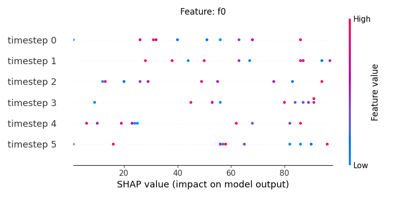
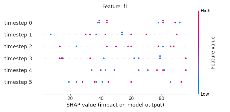
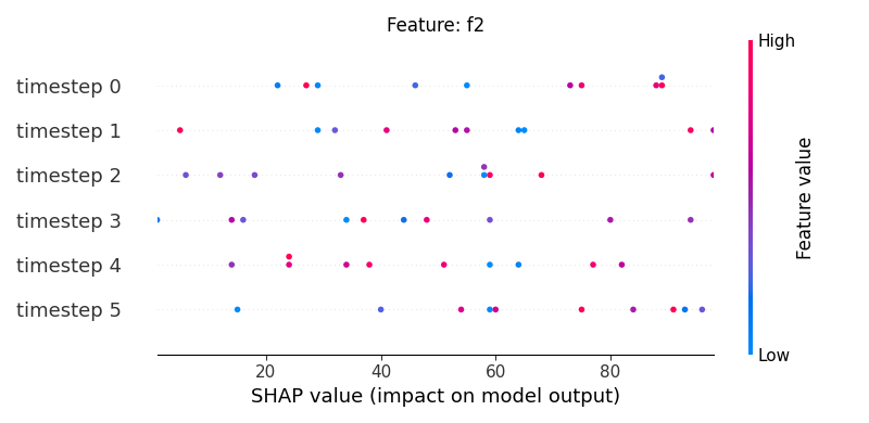
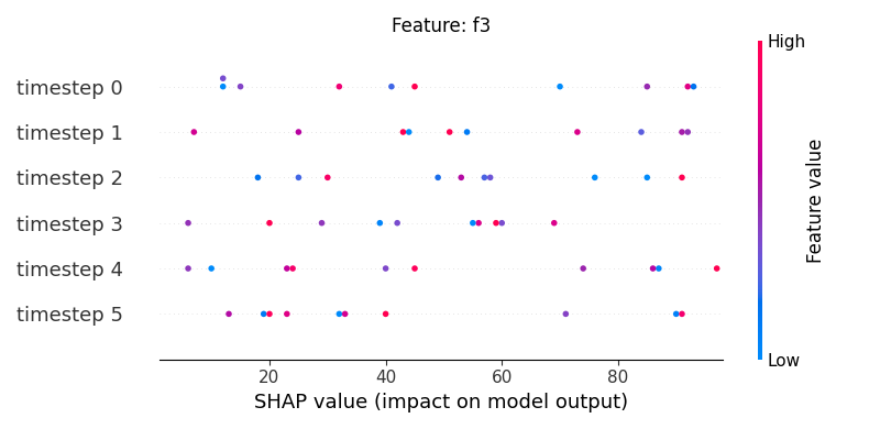
Note
If y-axis represents timesteps the sort parameter
in the summary_plot function is set to False.
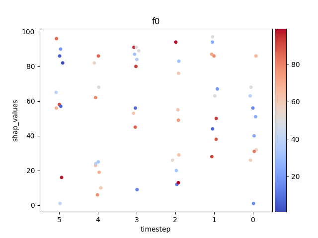
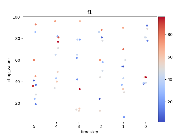
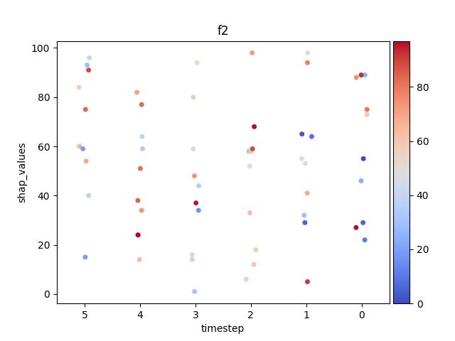
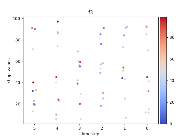
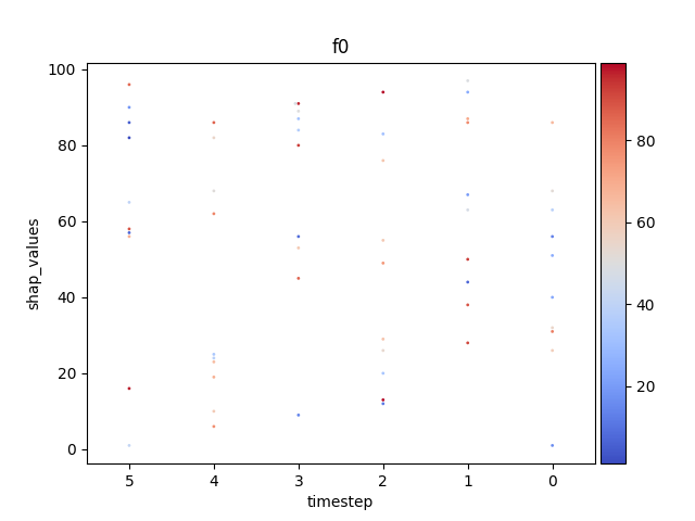
Display using sns.stripplot
Warning
This method seems to be quite slow.
Let’s display the shap values for each feature and all time steps. In contrast to the previous example, the timesteps are now displayed on the x-axis and the y-axis contains the shap values.
286 def add_colorbar(fig, cmap, norm):
287     """"""
288     divider = make_axes_locatable(plt.gca())
289     ax_cb = divider.new_horizontal(size="5%", pad=0.05)
290     fig.add_axes(ax_cb)
291     cb1 = matplotlib.colorbar.ColorbarBase(ax_cb,
292          cmap=cmap, norm=norm, orientation='vertical')
293
294
295 # Loop
296 for i, (name, df) in enumerate(data.groupby('features')):
297
298     # Get colormap
299     values = df.feature_values
300     cmap, norm = scalar_palette(values=values, cmap='coolwarm',
301         vmin=values.min(), vmax=values.max())
302
303     print(df)
304
305     # Display
306     fig, ax = plt.subplots()
307     ax = sns.stripplot(x='timestep',
308                        y='shap_values',
309                        hue='feature_values',
310                        palette=cmap,
311                        data=df,
312                        ax=ax)
313
314     # Needed for older matplotlib versions
315     cmap = matplotlib.cm.get_cmap('coolwarm')
316
317     # Configure axes
318     plt.title(name)
319     plt.legend([], [], frameon=False)
320     ax.invert_xaxis()
321     add_colorbar(plt.gcf(), cmap, norm)
322
323     # End
324     if int(i) > N:
325         break
326
327 # Show
328 plt.show()
Out:
sample timestep features shap_values feature_values
0 0 0 f0 61 65
4 0 1 f0 49 4
8 0 2 f0 68 0
12 0 3 f0 10 60
16 0 4 f0 11 61
20 0 5 f0 32 39
24 1 0 f0 53 36
28 1 1 f0 71 36
32 1 2 f0 74 6
36 1 3 f0 15 51
40 1 4 f0 56 13
44 1 5 f0 0 65
48 2 0 f0 24 66
52 2 1 f0 92 92
56 2 2 f0 50 15
60 2 3 f0 6 62
64 2 4 f0 43 45
68 2 5 f0 30 52
72 3 0 f0 28 36
76 3 1 f0 60 31
80 3 2 f0 26 64
84 3 3 f0 28 93
88 3 4 f0 82 29
92 3 5 f0 56 71
96 4 0 f0 37 68
100 4 1 f0 31 3
104 4 2 f0 57 95
108 4 3 f0 47 44
112 4 4 f0 89 52
116 4 5 f0 63 75
120 5 0 f0 30 86
124 5 1 f0 72 49
128 5 2 f0 20 40
132 5 3 f0 56 58
136 5 4 f0 64 26
140 5 5 f0 4 23
144 6 0 f0 20 85
148 6 1 f0 8 75
152 6 2 f0 50 93
156 6 3 f0 73 5
160 6 4 f0 98 98
164 6 5 f0 41 20
168 7 0 f0 45 80
172 7 1 f0 48 89
176 7 2 f0 31 51
180 7 3 f0 98 69
184 7 4 f0 3 5
188 7 5 f0 58 77
192 8 0 f0 26 18
196 8 1 f0 30 24
200 8 2 f0 92 72
204 8 3 f0 47 96
208 8 4 f0 9 45
212 8 5 f0 94 7
216 9 0 f0 64 86
220 9 1 f0 39 86
224 9 2 f0 27 13
228 9 3 f0 54 32
232 9 4 f0 4 54
236 9 5 f0 59 41
C:\Users\kelda\Desktop\repositories\github\python-spare-code\main\examples\shap\plot_main05.py:315: MatplotlibDeprecationWarning:
The get_cmap function was deprecated in Matplotlib 3.7 and will be removed in 3.11. Use ``matplotlib.colormaps[name]`` or ``matplotlib.colormaps.get_cmap()`` or ``pyplot.get_cmap()`` instead.
sample timestep features shap_values feature_values
1 0 0 f1 79 9
5 0 1 f1 66 71
9 0 2 f1 59 67
13 0 3 f1 7 85
17 0 4 f1 35 1
21 0 5 f1 62 94
25 1 0 f1 70 54
29 1 1 f1 31 40
33 1 2 f1 68 25
37 1 3 f1 99 6
41 1 4 f1 68 10
45 1 5 f1 66 4
49 2 0 f1 27 43
53 2 1 f1 64 69
57 2 2 f1 46 22
61 2 3 f1 92 38
65 2 4 f1 76 74
69 2 5 f1 92 11
73 3 0 f1 51 27
77 3 1 f1 99 52
81 3 2 f1 60 83
85 3 3 f1 34 65
89 3 4 f1 45 46
93 3 5 f1 86 88
97 4 0 f1 98 11
101 4 1 f1 2 46
105 4 2 f1 69 77
109 4 3 f1 14 55
113 4 4 f1 17 86
117 4 5 f1 90 0
121 5 0 f1 40 22
125 5 1 f1 65 93
129 5 2 f1 62 42
133 5 3 f1 67 50
137 5 4 f1 54 17
141 5 5 f1 45 69
145 6 0 f1 31 22
149 6 1 f1 44 45
153 6 2 f1 47 52
157 6 3 f1 1 8
161 6 4 f1 8 56
165 6 5 f1 27 79
169 7 0 f1 38 3
173 7 1 f1 53 7
177 7 2 f1 21 62
181 7 3 f1 34 62
185 7 4 f1 6 7
189 7 5 f1 12 41
193 8 0 f1 71 90
197 8 1 f1 81 82
201 8 2 f1 71 50
205 8 3 f1 41 12
209 8 4 f1 62 34
213 8 5 f1 96 93
217 9 0 f1 42 30
221 9 1 f1 35 52
225 9 2 f1 35 44
229 9 3 f1 51 56
233 9 4 f1 15 88
237 9 5 f1 4 19
C:\Users\kelda\Desktop\repositories\github\python-spare-code\main\examples\shap\plot_main05.py:315: MatplotlibDeprecationWarning:
The get_cmap function was deprecated in Matplotlib 3.7 and will be removed in 3.11. Use ``matplotlib.colormaps[name]`` or ``matplotlib.colormaps.get_cmap()`` or ``pyplot.get_cmap()`` instead.
sample timestep features shap_values feature_values
2 0 0 f2 10 46
6 0 1 f2 24 86
10 0 2 f2 34 50
14 0 3 f2 13 49
18 0 4 f2 3 59
22 0 5 f2 90 19
26 1 0 f2 92 90
30 1 1 f2 45 52
34 1 2 f2 72 79
38 1 3 f2 65 13
42 1 4 f2 38 74
46 1 5 f2 24 97
50 2 0 f2 75 1
54 2 1 f2 40 38
58 2 2 f2 34 7
62 2 3 f2 34 73
66 2 4 f2 1 65
70 2 5 f2 41 9
74 3 0 f2 5 12
78 3 1 f2 10 48
82 3 2 f2 64 97
86 3 3 f2 14 5
90 3 4 f2 51 32
94 3 5 f2 83 95
98 4 0 f2 82 88
102 4 1 f2 85 55
106 4 2 f2 12 68
110 4 3 f2 5 0
114 4 4 f2 34 60
118 4 5 f2 95 23
122 5 0 f2 52 1
126 5 1 f2 0 12
130 5 2 f2 46 39
134 5 3 f2 74 36
138 5 4 f2 8 6
142 5 5 f2 67 1
146 6 0 f2 2 41
150 6 1 f2 17 34
154 6 2 f2 25 62
158 6 3 f2 23 70
162 6 4 f2 19 52
166 6 5 f2 74 7
170 7 0 f2 18 66
174 7 1 f2 81 66
178 7 2 f2 87 98
182 7 3 f2 24 10
186 7 4 f2 76 28
190 7 5 f2 54 7
194 8 0 f2 88 85
198 8 1 f2 47 1
202 8 2 f2 76 87
206 8 3 f2 73 98
210 8 4 f2 82 97
214 8 5 f2 11 98
218 9 0 f2 57 39
222 9 1 f2 96 20
226 9 2 f2 86 45
230 9 3 f2 61 42
234 9 4 f2 32 3
238 9 5 f2 91 2
C:\Users\kelda\Desktop\repositories\github\python-spare-code\main\examples\shap\plot_main05.py:315: MatplotlibDeprecationWarning:
The get_cmap function was deprecated in Matplotlib 3.7 and will be removed in 3.11. Use ``matplotlib.colormaps[name]`` or ``matplotlib.colormaps.get_cmap()`` or ``pyplot.get_cmap()`` instead.
sample timestep features shap_values feature_values
3 0 0 f3 76 68
7 0 1 f3 38 32
11 0 2 f3 89 41
15 0 3 f3 68 82
19 0 4 f3 30 12
23 0 5 f3 89 8
27 1 0 f3 51 6
31 1 1 f3 27 74
35 1 2 f3 27 17
39 1 3 f3 82 70
43 1 4 f3 89 8
47 1 5 f3 42 74
51 2 0 f3 32 29
55 2 1 f3 87 64
59 2 2 f3 75 48
63 2 3 f3 99 94
67 2 4 f3 79 80
71 2 5 f3 51 66
75 3 0 f3 38 94
79 3 1 f3 54 56
83 3 2 f3 74 84
87 3 3 f3 46 22
91 3 4 f3 59 45
95 3 5 f3 59 82
99 4 0 f3 41 32
103 4 1 f3 76 46
107 4 2 f3 80 65
111 4 3 f3 87 61
115 4 4 f3 95 64
119 4 5 f3 49 46
123 5 0 f3 98 38
127 5 1 f3 55 50
131 5 2 f3 70 48
135 5 3 f3 74 47
139 5 4 f3 13 83
143 5 5 f3 59 52
147 6 0 f3 18 51
151 6 1 f3 9 5
155 6 2 f3 79 31
159 6 3 f3 67 48
163 6 4 f3 31 21
167 6 5 f3 43 44
171 7 0 f3 19 99
175 7 1 f3 77 10
179 7 2 f3 71 64
183 7 3 f3 80 37
187 7 4 f3 17 24
191 7 5 f3 30 95
195 8 0 f3 34 74
199 8 1 f3 45 6
203 8 2 f3 95 77
207 8 3 f3 84 30
211 8 4 f3 18 46
215 8 5 f3 40 90
219 9 0 f3 99 66
223 9 1 f3 29 23
227 9 2 f3 78 71
231 9 3 f3 95 59
235 9 4 f3 87 36
239 9 5 f3 27 4
C:\Users\kelda\Desktop\repositories\github\python-spare-code\main\examples\shap\plot_main05.py:315: MatplotlibDeprecationWarning:
The get_cmap function was deprecated in Matplotlib 3.7 and will be removed in 3.11. Use ``matplotlib.colormaps[name]`` or ``matplotlib.colormaps.get_cmap()`` or ``pyplot.get_cmap()`` instead.
C:\Users\kelda\Desktop\repositories\github\python-spare-code\main\examples\shap\plot_main05.py:328: UserWarning:
FigureCanvasAgg is non-interactive, and thus cannot be shown
Display using sns.swarmplot
Let’s display the shap values for each timestep.
342 # Loop
343 for i, (name, df) in enumerate(data.groupby('features')):
344
345     # Get colormap
346     values = df.feature_values
347     cmap, norm = scalar_palette(values=values, cmap='coolwarm',
348         vmin=values.min(), vmax=values.max())
349
350     # Display
351     fig, ax = plt.subplots()
352     ax = sns.swarmplot(x='timestep',
353                        y='shap_values',
354                        hue='feature_values',
355                        palette=cmap,
356                        data=df,
357                        size=2,
358                        ax=ax)
359
360     # Needed for older matplotlib versions
361     cmap = matplotlib.cm.get_cmap('coolwarm')
362
363     # Configure axes
364     plt.title(name)
365     plt.legend([], [], frameon=False)
366     ax.invert_xaxis()
367     add_colorbar(plt.gcf(), cmap, norm)
368
369     # End
370     if int(i) > N:
371         break
372
373 # Show
374 plt.show()
375
376
377
378
379
380
381
382 """
383 sns.set_theme(style="ticks")
384
385 # Create a dataset with many short random walks
386 rs = np.random.RandomState(4)
387 pos = rs.randint(-1, 2, (20, 5)).cumsum(axis=1)
388 pos -= pos[:, 0, np.newaxis]
389 step = np.tile(range(5), 20)
390 walk = np.repeat(range(20), 5)
391 df = pd.DataFrame(np.c_[pos.flat, step, walk],
392                   columns=["position", "step", "walk"])
393 # Initialize a grid of plots with an Axes for each walk
394 #grid = sns.FacetGrid(df_stack, col="walk", hue="f", palette="tab20c",
395 #                     col_wrap=4, height=1.5)
396
397 grid = sns.FacetGrid(df_stack, hue="f",
398     palette="tab20c", height=1.5)
399
400 # Draw a horizontal line to show the starting point
401 grid.refline(y=0, linestyle=":")
402
403 # Draw a line plot to show the trajectory of each random walk
404 grid.map(plt.plot, "t", "value", marker="o")
405
406 # Adjust the tick positions and labels
407 grid.set(xticks=np.arange(5), yticks=[-3, 3],
408          xlim=(-.5, 4.5), ylim=(-3.5, 3.5))
409
410 # Adjust the arrangement of the plots
411 grid.fig.tight_layout(w_pad=1)
412
413 """
414
415
416 #plt.show()
Out:
C:\Users\kelda\Desktop\repositories\github\python-spare-code\main\examples\shap\plot_main05.py:361: MatplotlibDeprecationWarning:

The get_cmap function was deprecated in Matplotlib 3.7 and will be removed in 3.11. Use ``matplotlib.colormaps[name]`` or ``matplotlib.colormaps.get_cmap()`` or ``pyplot.get_cmap()`` instead.

C:\Users\kelda\Desktop\repositories\github\python-spare-code\main\examples\shap\plot_main05.py:374: UserWarning:

FigureCanvasAgg is non-interactive, and thus cannot be shown


'\nsns.set_theme(style="ticks")\n\n# Create a dataset with many short random walks\nrs = np.random.RandomState(4)\npos = rs.randint(-1, 2, (20, 5)).cumsum(axis=1)\npos -= pos[:, 0, np.newaxis]\nstep = np.tile(range(5), 20)\nwalk = np.repeat(range(20), 5)\ndf = pd.DataFrame(np.c_[pos.flat, step, walk],\n                  columns=["position", "step", "walk"])\n# Initialize a grid of plots with an Axes for each walk\n#grid = sns.FacetGrid(df_stack, col="walk", hue="f", palette="tab20c",\n#                     col_wrap=4, height=1.5)\n\ngrid = sns.FacetGrid(df_stack, hue="f",\n    palette="tab20c", height=1.5)\n\n# Draw a horizontal line to show the starting point\ngrid.refline(y=0, linestyle=":")\n\n# Draw a line plot to show the trajectory of each random walk\ngrid.map(plt.plot, "t", "value", marker="o")\n\n# Adjust the tick positions and labels\ngrid.set(xticks=np.arange(5), yticks=[-3, 3],\n         xlim=(-.5, 4.5), ylim=(-3.5, 3.5))\n\n# Adjust the arrangement of the plots\ngrid.fig.tight_layout(w_pad=1)\n\n'
Display using sns.FacetGrid
423 #g = sns.FacetGrid(df_stack, col="f", hue='original')
424 #g.map(sns.swarmplot, "t", "value", alpha=.7)
425 #g.add_legend()
Display using shap.beeswarm
433 # REF: https://github.com/slundberg/shap/blob/master/shap/plots/_beeswarm.py
434 #
435 # .. note: It needs a kernel explainer, and while it works with
436 #          common kernels (plot_main07.py) it does not work with
437 #          the DeepKernel for some reason (mask related).
Total running time of the script: ( 0 minutes 3.032 seconds)