Note
Click here to download the full example code
05b. Custom using summary_plot
This script demonstrates how to adapt the standard shap.summary_plot
for visualizing the complex, three-dimensional SHAP values
(samples, timesteps, features) generated by sequential models.
It provides a powerful strategy for interpreting feature importance
both at specific points in time and across an entire sequence.
The script showcases a two-pronged visualization approach:
Data Reshaping: It begins by pivoting a tidy DataFrame into the wide-format matrices for SHAP values and feature values that are required by the plotting function.
Per-Timestep Analysis: It first iterates through each timestep, creating a separate summary plot that reveals the importance of all features at that single moment in the sequence.
Per-Feature Analysis: It then iterates through each feature, generating a summary plot that visualizes how the importance of that single feature evolves across all timesteps.
This example is essential for effectively using SHAP’s most common plot to uncover the temporal dynamics of feature contributions in time-series and sequential data models.
29 # Libraries
30 import shap
31 import pandas as pd
32
33 import matplotlib.pyplot as plt
34
35
36 try:
37     __file__
38     TERMINAL = True
39 except:
40     TERMINAL = False
41
42
43 # ------------------------
44 # Methods
45 # ------------------------
46 def load_shap_file():
47     """Load shap file.
48
49     .. note: The timestep does not indicate time step but matrix
50              index index. Since the matrix index for time steps
51              started in negative t=-T and ended in t=0 the
52              transformation should be taken into account.
53
54     """
55     from pathlib import Path
56     # Load data
57     path = Path('../../datasets/shap/')
58     data = pd.read_csv(path / 'shap.csv')
59     data = data.iloc[:, 1:]
60     data = data.rename(columns={'timestep': 'indice'})
61     data['timestep'] = data.indice - (data.indice.nunique() - 1)
62     return data
63
64
65 # -----------------------------------------------------
66 #                       Main
67 # -----------------------------------------------------
68 # Load data
69 # data = create_random_shap(10, 6, 4)
70 data = load_shap_file()
71 #data = data[data['sample'] < 100]
72
73 shap_values = pd.pivot_table(data,
74                              values='shap_values',
75                              index=['sample', 'timestep'],
76                              columns=['features'])
77
78 feature_values = pd.pivot_table(data,
79                                 values='feature_values',
80                                 index=['sample', 'timestep'],
81                                 columns=['features'])
82
83 # Show
84 if TERMINAL:
85     print("\nShow:")
86     print(data)
87     print(shap_values)
88     print(feature_values)
Let’s see how data looks like
92 data.head(10)
Let’s see how shap_values looks like
96 shap_values.iloc[:10, :5]
Let’s see how feature_values looks like
100 feature_values.iloc[:10, :5]
Display using shap.summary_plot
105 #
106 # The first option is to use the ``shap`` library to plot the results.
107
108 # Let's define/extract some useful variables.
109 N = 10  # max loops filter
110 TIMESTEPS = len(shap_values.index.unique(level='timestep'))  # number of timesteps
111 SAMPLES = len(shap_values.index.unique(level='sample'))  # number of samples
112
113 shap_min = data.shap_values.min()
114 shap_max = data.shap_values.max()
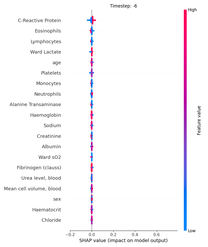
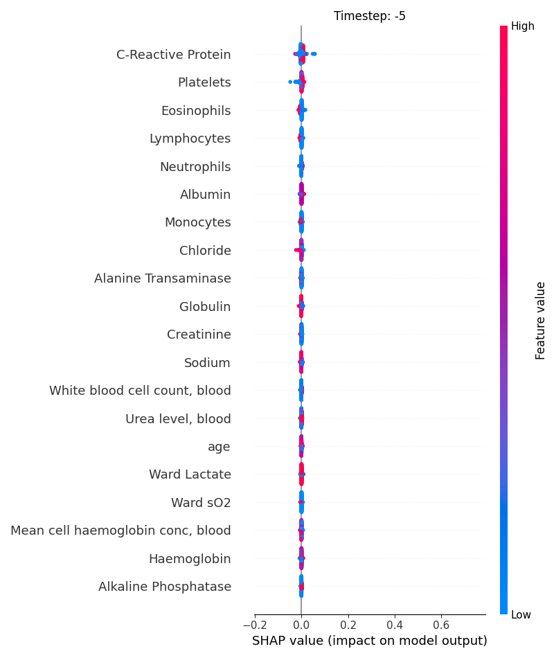
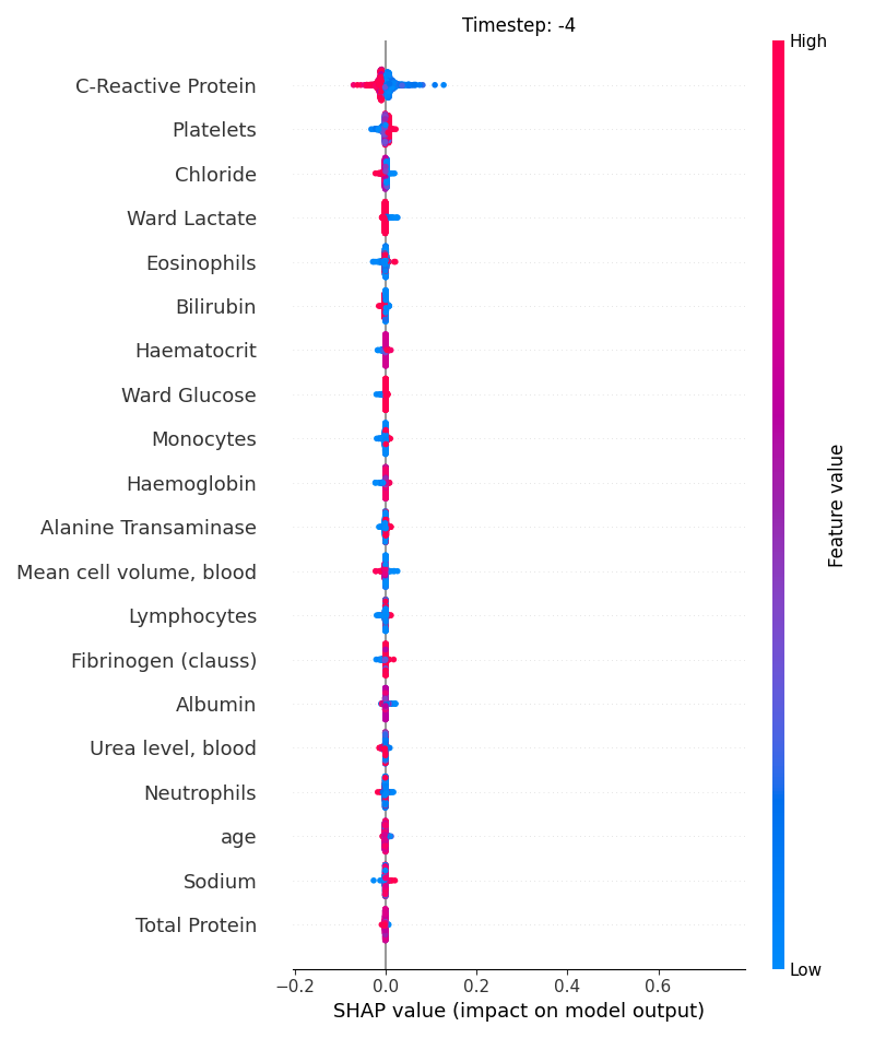
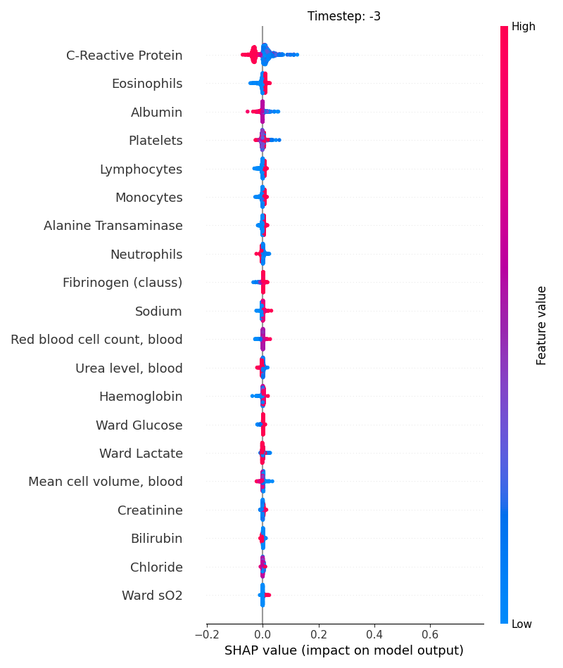
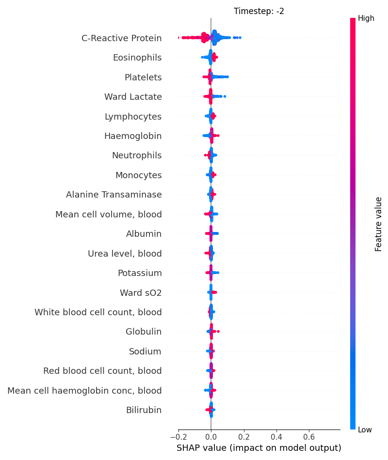
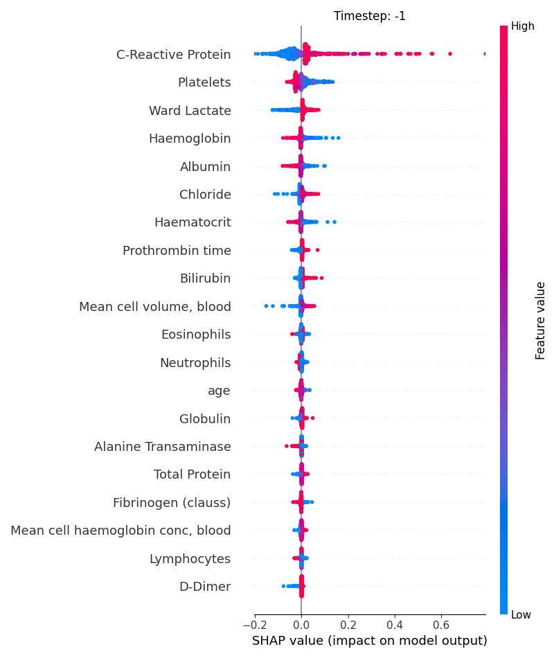
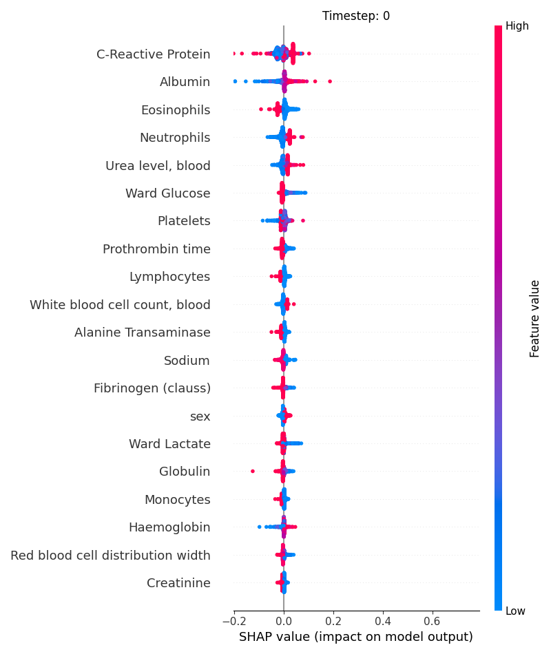
Now, let’s display the shap values for all features in each timestep.
121 # For each timestep (visualise all features)
122 steps = shap_values.index.get_level_values('timestep').unique()
123 for i, step in enumerate(steps):
124     # Get interesting indexes
125     indice = shap_values.index.get_level_values('timestep') == step
126
127     # Create auxiliary matrices
128     shap_aux = shap_values.iloc[indice]
129     feat_aux = feature_values.iloc[indice]
130
131     # Display
132     plt.figure()
133     plt.title("Timestep: %s" % step)
134     shap.summary_plot(shap_aux.to_numpy(), feat_aux, show=False)
135     plt.xlim(shap_min, shap_max)
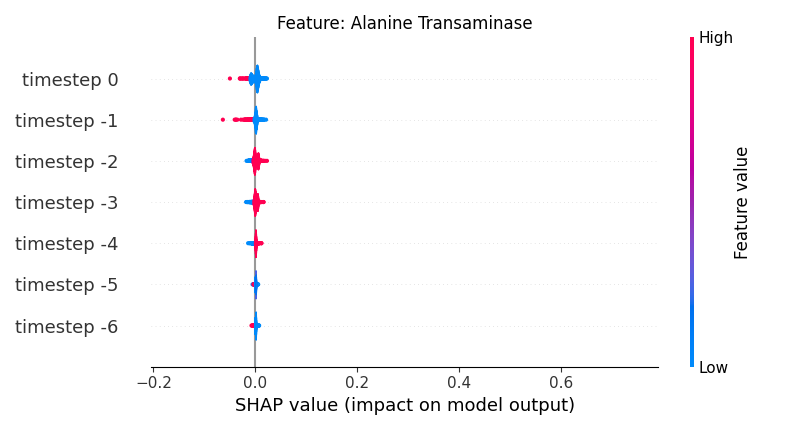
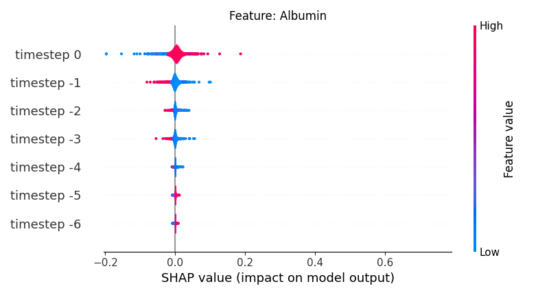
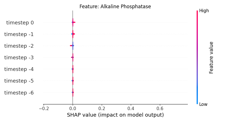
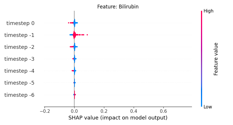
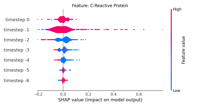
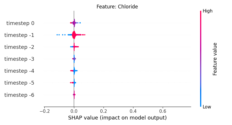
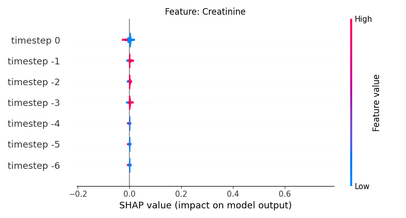
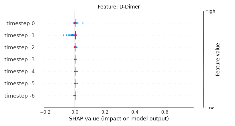
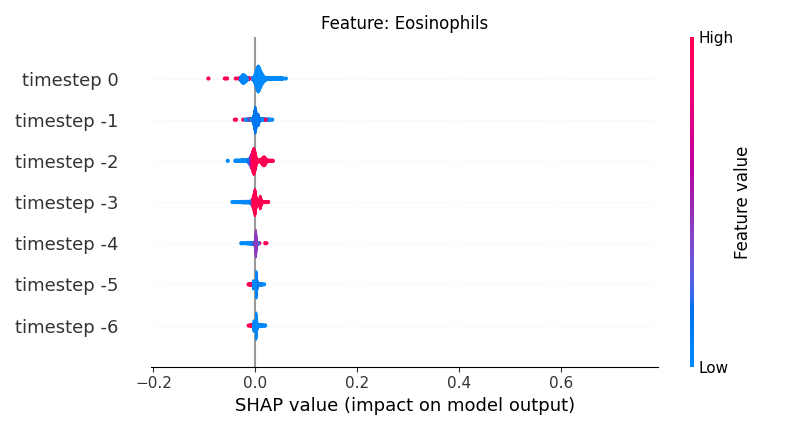
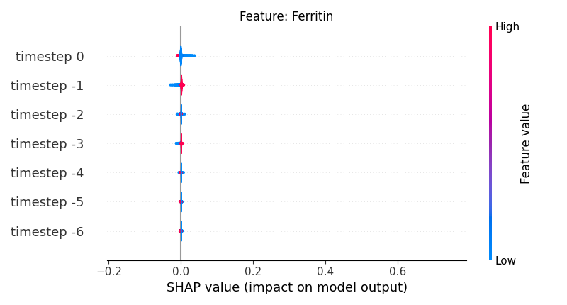
Now, let’s display the shap values for all timesteps of each feature.
141 # For each feature (visualise all time-steps)
142 for i, f in enumerate(shap_values.columns[:N]):
143     # Show
144     # print('%2d. %s' % (i, f))
145
146     # Create auxiliary matrices (select feature and reshape)
147     shap_aux = shap_values.iloc[:, i] \
148         .to_numpy().reshape(-1, TIMESTEPS)
149     feat_aux = feature_values.iloc[:, i] \
150         .to_numpy().reshape(-1, TIMESTEPS)
151     feat_aux = pd.DataFrame(feat_aux,
152         columns=['timestep %s' % j for j in range(-TIMESTEPS+1, 1)]
153         )
154
155     # Show
156     plt.figure()
157     plt.title("Feature: %s" % f)
158     shap.summary_plot(shap_aux, feat_aux, sort=False, show=False, plot_type='violin')
159     plt.xlim(shap_min, shap_max)
160     plt.gca().invert_yaxis()
161
162 # Show
163 plt.show()
Out:
C:\Users\kelda\Desktop\repositories\github\python-spare-code\main\examples\shap\plot_main05_summaryplot.py:163: UserWarning:

FigureCanvasAgg is non-interactive, and thus cannot be shown
Total running time of the script: ( 0 minutes 8.284 seconds)