Note
Click here to download the full example code
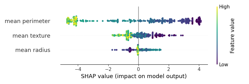
12b. Matplotlib to Plotly (shap)
This example converts a matplotlib figure to Plotly.
Warning
A known bug in Plotly (see GitHub issue) causes the mpl_to_plotly() function to fail because it references an outdated function from Matplotlib. The current fix is to downgrade to an older version of Matplotlib or to recreate your figure in Plotly manually.
[ISSUE]: https://github.com/plotly/plotly.py/issues/3624#issuecomment-1161805210 In the latest commit of plotly packages/python/plotly/plotly/matplotlylib/mpltools.py line 368, it still calls is_frame_like() function.
Note
In the latest commit of plotly packages/python/plotly/plotly/matplotlylib/mpltools.py line 368, it still calls is_frame_like() function. There is already an issue tracking this. You may need choose to downgrade Matplotlib if you still want to use mpl_to_plotly() function.
Out:
Kernel type: <class 'shap.explainers._tree.TreeExplainer'>
Shap values:
.values =
array([[-0.07339976,  1.23534454, -4.69448856],
       [-0.28925516, -0.13902985, -4.83976683],
       [-0.23044579, -0.75952114, -4.40960412],
       ...,
       [ 0.41172362,  0.30341838,  1.756622  ],
       [-0.28925516, -0.13902985, -4.83976683],
       [-0.23044579, -0.75952114, -4.40960412]])

.base_values =
array([0.80274342, 0.80274342, 0.80274342, 0.80274342, 0.80274342,
       0.80274342, 0.80274342, 0.80274342, 0.80274342, 0.80274342,
       0.80274342, 0.80274342, 0.80274342, 0.80274342, 0.80274342,
       0.80274342, 0.80274342, 0.80274342, 0.80274342, 0.80274342,
       0.80274342, 0.80274342, 0.80274342, 0.80274342, 0.80274342,
       0.80274342, 0.80274342, 0.80274342, 0.80274342, 0.80274342,
       0.80274342, 0.80274342, 0.80274342, 0.80274342, 0.80274342,
       0.80274342, 0.80274342, 0.80274342, 0.80274342, 0.80274342,
       0.80274342, 0.80274342, 0.80274342, 0.80274342, 0.80274342,
       0.80274342, 0.80274342, 0.80274342, 0.80274342, 0.80274342,
       0.80274342, 0.80274342, 0.80274342, 0.80274342, 0.80274342,
       0.80274342, 0.80274342, 0.80274342, 0.80274342, 0.80274342,
       0.80274342, 0.80274342, 0.80274342, 0.80274342, 0.80274342,
       0.80274342, 0.80274342, 0.80274342, 0.80274342, 0.80274342,
       0.80274342, 0.80274342, 0.80274342, 0.80274342, 0.80274342,
       0.80274342, 0.80274342, 0.80274342, 0.80274342, 0.80274342,
       0.80274342, 0.80274342, 0.80274342, 0.80274342, 0.80274342,
       0.80274342, 0.80274342, 0.80274342, 0.80274342, 0.80274342,
       0.80274342, 0.80274342, 0.80274342, 0.80274342, 0.80274342,
       0.80274342, 0.80274342, 0.80274342, 0.80274342, 0.80274342,
       0.80274342, 0.80274342, 0.80274342, 0.80274342, 0.80274342,
       0.80274342, 0.80274342, 0.80274342, 0.80274342, 0.80274342,
       0.80274342, 0.80274342, 0.80274342, 0.80274342, 0.80274342,
       0.80274342, 0.80274342, 0.80274342, 0.80274342, 0.80274342,
       0.80274342, 0.80274342, 0.80274342, 0.80274342, 0.80274342,
       0.80274342, 0.80274342, 0.80274342, 0.80274342, 0.80274342,
       0.80274342, 0.80274342, 0.80274342, 0.80274342, 0.80274342,
       0.80274342, 0.80274342, 0.80274342, 0.80274342, 0.80274342,
       0.80274342, 0.80274342, 0.80274342, 0.80274342, 0.80274342,
       0.80274342, 0.80274342, 0.80274342, 0.80274342, 0.80274342,
       0.80274342, 0.80274342, 0.80274342, 0.80274342, 0.80274342,
       0.80274342, 0.80274342, 0.80274342, 0.80274342, 0.80274342,
       0.80274342, 0.80274342, 0.80274342, 0.80274342, 0.80274342,
       0.80274342, 0.80274342, 0.80274342, 0.80274342, 0.80274342,
       0.80274342, 0.80274342, 0.80274342, 0.80274342, 0.80274342,
       0.80274342, 0.80274342, 0.80274342, 0.80274342, 0.80274342,
       0.80274342, 0.80274342, 0.80274342, 0.80274342, 0.80274342,
       0.80274342, 0.80274342, 0.80274342, 0.80274342, 0.80274342,
       0.80274342, 0.80274342, 0.80274342, 0.80274342, 0.80274342,
       0.80274342, 0.80274342, 0.80274342, 0.80274342, 0.80274342,
       0.80274342, 0.80274342, 0.80274342, 0.80274342, 0.80274342,
       0.80274342, 0.80274342, 0.80274342, 0.80274342, 0.80274342,
       0.80274342, 0.80274342, 0.80274342, 0.80274342, 0.80274342,
       0.80274342, 0.80274342, 0.80274342, 0.80274342, 0.80274342,
       0.80274342, 0.80274342, 0.80274342, 0.80274342, 0.80274342,
       0.80274342, 0.80274342, 0.80274342, 0.80274342, 0.80274342,
       0.80274342, 0.80274342, 0.80274342, 0.80274342, 0.80274342,
       0.80274342, 0.80274342, 0.80274342, 0.80274342, 0.80274342,
       0.80274342, 0.80274342, 0.80274342, 0.80274342, 0.80274342,
       0.80274342, 0.80274342, 0.80274342, 0.80274342, 0.80274342,
       0.80274342, 0.80274342, 0.80274342, 0.80274342, 0.80274342,
       0.80274342, 0.80274342, 0.80274342, 0.80274342, 0.80274342,
       0.80274342, 0.80274342, 0.80274342, 0.80274342, 0.80274342,
       0.80274342, 0.80274342, 0.80274342, 0.80274342, 0.80274342,
       0.80274342, 0.80274342, 0.80274342, 0.80274342, 0.80274342,
       0.80274342, 0.80274342, 0.80274342, 0.80274342, 0.80274342,
       0.80274342, 0.80274342, 0.80274342, 0.80274342, 0.80274342,
       0.80274342, 0.80274342, 0.80274342, 0.80274342, 0.80274342,
       0.80274342, 0.80274342, 0.80274342, 0.80274342, 0.80274342,
       0.80274342, 0.80274342, 0.80274342, 0.80274342, 0.80274342,
       0.80274342, 0.80274342, 0.80274342, 0.80274342, 0.80274342,
       0.80274342, 0.80274342, 0.80274342, 0.80274342, 0.80274342,
       0.80274342, 0.80274342, 0.80274342, 0.80274342, 0.80274342,
       0.80274342, 0.80274342, 0.80274342, 0.80274342, 0.80274342,
       0.80274342, 0.80274342, 0.80274342, 0.80274342, 0.80274342,
       0.80274342, 0.80274342, 0.80274342, 0.80274342, 0.80274342,
       0.80274342, 0.80274342, 0.80274342, 0.80274342, 0.80274342,
       0.80274342, 0.80274342, 0.80274342, 0.80274342, 0.80274342,
       0.80274342, 0.80274342, 0.80274342, 0.80274342, 0.80274342,
       0.80274342, 0.80274342, 0.80274342, 0.80274342, 0.80274342,
       0.80274342, 0.80274342, 0.80274342, 0.80274342, 0.80274342,
       0.80274342, 0.80274342, 0.80274342, 0.80274342, 0.80274342,
       0.80274342, 0.80274342, 0.80274342, 0.80274342, 0.80274342,
       0.80274342, 0.80274342, 0.80274342, 0.80274342, 0.80274342,
       0.80274342, 0.80274342, 0.80274342, 0.80274342, 0.80274342,
       0.80274342, 0.80274342, 0.80274342, 0.80274342, 0.80274342,
       0.80274342, 0.80274342, 0.80274342, 0.80274342, 0.80274342,
       0.80274342, 0.80274342, 0.80274342, 0.80274342, 0.80274342,
       0.80274342, 0.80274342, 0.80274342, 0.80274342, 0.80274342,
       0.80274342, 0.80274342, 0.80274342, 0.80274342, 0.80274342,
       0.80274342, 0.80274342, 0.80274342, 0.80274342, 0.80274342,
       0.80274342, 0.80274342, 0.80274342, 0.80274342, 0.80274342,
       0.80274342, 0.80274342, 0.80274342, 0.80274342, 0.80274342,
       0.80274342, 0.80274342, 0.80274342, 0.80274342, 0.80274342,
       0.80274342, 0.80274342, 0.80274342, 0.80274342, 0.80274342,
       0.80274342, 0.80274342, 0.80274342, 0.80274342, 0.80274342,
       0.80274342, 0.80274342, 0.80274342, 0.80274342, 0.80274342,
       0.80274342, 0.80274342, 0.80274342, 0.80274342, 0.80274342,
       0.80274342, 0.80274342, 0.80274342, 0.80274342, 0.80274342,
       0.80274342, 0.80274342, 0.80274342, 0.80274342, 0.80274342,
       0.80274342, 0.80274342, 0.80274342, 0.80274342, 0.80274342,
       0.80274342, 0.80274342, 0.80274342, 0.80274342, 0.80274342,
       0.80274342, 0.80274342, 0.80274342, 0.80274342, 0.80274342,
       0.80274342, 0.80274342, 0.80274342, 0.80274342, 0.80274342,
       0.80274342, 0.80274342, 0.80274342, 0.80274342, 0.80274342,
       0.80274342, 0.80274342, 0.80274342, 0.80274342, 0.80274342,
       0.80274342, 0.80274342, 0.80274342, 0.80274342, 0.80274342,
       0.80274342, 0.80274342, 0.80274342, 0.80274342, 0.80274342,
       0.80274342, 0.80274342, 0.80274342, 0.80274342, 0.80274342,
       0.80274342, 0.80274342, 0.80274342, 0.80274342, 0.80274342])

.data =
array([[ 17.99,  10.38, 122.8 ],
       [ 20.57,  17.77, 132.9 ],
       [ 19.69,  21.25, 130.  ],
       ...,
       [ 12.47,  17.31,  80.45],
       [ 18.49,  17.52, 121.3 ],
       [ 20.59,  21.24, 137.8 ]])
(500, 3)
(500,)
(500, 3)

'\n# Convert to plotly\nimport plotly.tools as tls\nimport plotly.graph_objs as go\n\n# Get current figure and convert\nfig = tls.mpl_to_plotly(plt.gcf())\n\n# Format\n# Update layout\nfig.update_layout(\n    #xaxis_title=\'False Positive Rate\',\n    #yaxis_title=\'True Positive Rate\',\n    #yaxis=dict(scaleanchor="x", scaleratio=1),\n    #xaxis=dict(constrain=\'domain\'),\n    width=700, height=350,\n    #legend=dict(\n    #    x=1.0, y=0.0,  # x=1, y=1.02\n    #    orientation="v",\n    #    font=dict(\n    #       size=12,\n    #        color=\'black\'),\n    #    yanchor="bottom",\n    #    xanchor="right",\n    #),\n    font=dict(\n        size=15,\n        #family="Times New Roman",\n        #color="black",\n    ),\n    title=dict(\n        font=dict(\n        #    family="Times New Roman",\n        #    color="black"\n        )\n    ),\n    yaxis=dict(\n        tickmode=\'array\',\n        tickvals=[0, 1, 2],\n        ticktext=features[:-1],\n        tickfont=dict(size=15)\n    ),\n    xaxis=dict(\n        tickfont=dict(size=15)),\n    #margin={\n    #    \'l\': 0,\n    #    \'r\': 0,\n    #    \'b\': 0,\n    #    \'t\': 0,\n    #    \'pad\': 4\n    #},\n    paper_bgcolor=\'rgba(0,0,0,0)\',  # transparent\n    plot_bgcolor=\'rgba(0,0,0,0)\',   # transparent\n    template=\'simple_white\'\n)\n\n# Update scatter\nfig.update_traces(marker={\'size\': 10})\n\n# Add vertical lin\nfig.add_vline(x=0.0, line_width=2,\n    line_dash="dash", line_color="black") # green\n\n# .. note:: Would it be possible to get the values of\n#           cmin, cmax and the tick vals from the shap\n#           values? Ideally we do not want to hardcode\n#           them.\n\n# Add colorbar\ncolorbar_trace = go.Scatter(\n    x=[None], y=[None], mode=\'markers\',\n    marker=dict(\n        colorscale=\'viridis\',\n        showscale=True,\n        cmin=-5,\n        cmax=5,\n        colorbar=dict(thickness=20,\n            tickvals=[-5, 5],\n            ticktext=[\'Low\', \'High\'],\n            outlinewidth=0)),\n    hoverinfo=\'none\'\n)\nfig[\'layout\'][\'showlegend\'] = False\nfig.add_trace(colorbar_trace)\n\n# Show\n#fig.show()\nfig\n'
 22 # Generic
 23 import numpy as np
 24 import pandas as pd
 25 import matplotlib.pyplot as plt
 26
 27 # Sklearn
 28 from sklearn.model_selection import train_test_split
 29 from sklearn.datasets import load_iris
 30 from sklearn.datasets import load_breast_cancer
 31 from sklearn.naive_bayes import GaussianNB
 32 from sklearn.linear_model import LogisticRegression
 33 from sklearn.tree import DecisionTreeClassifier
 34 from sklearn.ensemble import RandomForestClassifier
 35
 36 # Xgboost
 37 from xgboost import XGBClassifier
 38
 39 try:
 40     __file__
 41     TERMINAL = True
 42 except:
 43     TERMINAL = False
 44
 45
 46 # ----------------------------------------
 47 # Load data
 48 # ----------------------------------------
 49 # Seed
 50 seed = 0
 51
 52 # Load dataset
 53 bunch = load_iris()
 54 bunch = load_breast_cancer()
 55
 56 # Features
 57 features = list(bunch['feature_names'])
 58
 59 # Create DataFrame
 60 data = pd.DataFrame(data=np.c_[bunch['data'],
 61     bunch['target']], columns=features + ['target'])
 62
 63 # Create X, y
 64 X = data[bunch['feature_names']]
 65 y = data['target']
 66
 67 # Filter
 68 X = X.iloc[:500, :3]
 69 y = y.iloc[:500]
 70
 71 # Split dataset
 72 X_train, X_test, y_train, y_test = \
 73     train_test_split(X, y, random_state=seed)
 74
 75
 76 # ----------------------------------------
 77 # Classifiers
 78 # ----------------------------------------
 79 # Define some classifiers
 80 gnb = GaussianNB()
 81 llr = LogisticRegression()
 82 dtc = DecisionTreeClassifier(random_state=seed)
 83 rfc = RandomForestClassifier(random_state=seed)
 84 xgb = XGBClassifier(
 85     min_child_weight=0.005,
 86     eta= 0.05, gamma= 0.2,
 87     max_depth= 4,
 88     n_estimators= 100)
 89
 90 # Select one
 91 clf = xgb
 92
 93 # Fit
 94 clf.fit(X_train, y_train)
 95
 96 # ----------------------------------------
 97 # Compute shap values
 98 # ----------------------------------------
 99 # Import
100 import shap
101
102 # Get generic explainer
103 explainer = shap.Explainer(clf, X_train)
104
105 # Show kernel type
106 print("\nKernel type: %s" % type(explainer))
107
108 # Get shap values
109 shap_values = explainer(X)
110
111 # Show shap values
112 print("Shap values:")
113 print(shap_values)
114 print(shap_values.values.shape)
115 print(shap_values.base_values.shape)
116 print(shap_values.data.shape)
117
118 # Get matplotlib figure
119 plot_summary = shap.summary_plot( \
120     explainer.shap_values(X_train),
121     X_train, cmap='viridis',
122     show=False)
123
124 # Show
125 #plt.show()
126
127 """
128 # Convert to plotly
129 import plotly.tools as tls
130 import plotly.graph_objs as go
131
132 # Get current figure and convert
133 fig = tls.mpl_to_plotly(plt.gcf())
134
135 # Format
136 # Update layout
137 fig.update_layout(
138     #xaxis_title='False Positive Rate',
139     #yaxis_title='True Positive Rate',
140     #yaxis=dict(scaleanchor="x", scaleratio=1),
141     #xaxis=dict(constrain='domain'),
142     width=700, height=350,
143     #legend=dict(
144     #    x=1.0, y=0.0,  # x=1, y=1.02
145     #    orientation="v",
146     #    font=dict(
147     #       size=12,
148     #        color='black'),
149     #    yanchor="bottom",
150     #    xanchor="right",
151     #),
152     font=dict(
153         size=15,
154         #family="Times New Roman",
155         #color="black",
156     ),
157     title=dict(
158         font=dict(
159         #    family="Times New Roman",
160         #    color="black"
161         )
162     ),
163     yaxis=dict(
164         tickmode='array',
165         tickvals=[0, 1, 2],
166         ticktext=features[:-1],
167         tickfont=dict(size=15)
168     ),
169     xaxis=dict(
170         tickfont=dict(size=15)),
171     #margin={
172     #    'l': 0,
173     #    'r': 0,
174     #    'b': 0,
175     #    't': 0,
176     #    'pad': 4
177     #},
178     paper_bgcolor='rgba(0,0,0,0)',  # transparent
179     plot_bgcolor='rgba(0,0,0,0)',   # transparent
180     template='simple_white'
181 )
182
183 # Update scatter
184 fig.update_traces(marker={'size': 10})
185
186 # Add vertical lin
187 fig.add_vline(x=0.0, line_width=2,
188     line_dash="dash", line_color="black") # green
189
190 # .. note:: Would it be possible to get the values of
191 #           cmin, cmax and the tick vals from the shap
192 #           values? Ideally we do not want to hardcode
193 #           them.
194
195 # Add colorbar
196 colorbar_trace = go.Scatter(
197     x=[None], y=[None], mode='markers',
198     marker=dict(
199         colorscale='viridis',
200         showscale=True,
201         cmin=-5,
202         cmax=5,
203         colorbar=dict(thickness=20,
204             tickvals=[-5, 5],
205             ticktext=['Low', 'High'],
206             outlinewidth=0)),
207     hoverinfo='none'
208 )
209 fig['layout']['showlegend'] = False
210 fig.add_trace(colorbar_trace)
211
212 # Show
213 #fig.show()
214 fig
215 """
Total running time of the script: ( 0 minutes 1.883 seconds)